Anthropogenic Heat in Urban Climate Systems: Forcing, Sensitivity, and Feedback
- Department of Earth and Environment, Boston University, Boston, USA
- Department of Mechanical Engineering, Boston University, Boston, USA
- Department of Transdisciplinary Science and Engineering, Institute of Science Tokyo, Tokyo, Japan
- Department of Risk and Disaster Reduction, University College London, London, UK
- Center for Climate Change Adaptation, National Institute for Environmental Studies, Tsukuba, Japan
- Department of Civil and Environmental Engineering, Hong Kong University of Science and Technology, Hong Kong, China
- School of Geographical Sciences and Urban Planning, Arizona State University, Phoenix, USA
Corresponding author: Dan Li ([email protected])
Abstract
Anthropogenic heat flux, the heat released to the environment from human activities such as building energy use, transportation, industrial processes, and human metabolism, is a defining feature of the urban climate system. It is an important contributor to the urban heat island (UHI) effect and influences a wide range of urban meteorological processes. Its significance extends beyond urban climatology because of its close connections to energy consumption, greenhouse gas emissions, and climate adaptation. Despite decades of research, anthropogenic heat flux remains one of the least well-constrained components of the urban energy balance. Moreover, its climatic significance has often been assessed from an applied perspective, with less emphasis on developing transferable physical understanding of how anthropogenic heat flux acts as a forcing, how urban temperatures respond, and how feedbacks modify that response. This review develops a forcing–response–feedback framework for synthesizing current understanding of the role of anthropogenic heat flux in the urban climate system and identifies priorities for future research.
Plain language summary
Cities release large amounts of heat into the environment through buildings, transportation, industry, and human metabolism. This anthropogenic heat contributes to urban warming, influences weather and climate, and is closely linked to energy demand and climate adaptation. Despite decades of research, a unified framework for understanding its climatic effects has been lacking. This review develops a forcing–response–feedback framework showing that the climatic impact of anthropogenic heat flux depends not only on its magnitude, but also on the temperature sensitivity to this forcing and on feedbacks that modulate that sensitivity. We distinguish different definitions of sensitivity and feedback, review advances and uncertainties in estimating anthropogenic heat flux, synthesize observational and modeling evidence for both temperature sensitivity and feedback processes, and identify priorities for future research.
Key points
- A unified forcing–response–feedback framework is developed for understanding the climatic impacts of anthropogenic heat flux.
- The literature on anthropogenic heat flux and its climatic impacts is synthesized using this unified framework.
- Major uncertainties and gaps in anthropogenic heat flux research are identified.
Introduction
Long before the emergence of contemporary climate science, scientists had already begun to consider whether the heat released from human energy consumption during urbanization and industrialization could influence weather and climate. One of the earliest discussions of this idea appeared in Luke Howard’s The Climate of London (Howard 1833). Howard was the first to document what is now known as the urban heat island (UHI) effect, the tendency for cities to be warmer than their surrounding rural areas, and to postulate that the UHI effect was associated with the heat released from human metabolism, domestic heating, industrial activity, and combustion sources throughout the city. Howard even remarked that “the real matter of surprise, when we contemplate so many sources of heat in a city is, that the effect on the thermometer is not more considerable.” The heat sources identified by Howard are now commonly referred to collectively as anthropogenic heat flux (\(Q_F\)). Throughout this review, the terms anthropogenic heat flux, anthropogenic heat emissions, anthropogenic heat release, anthropogenic heating, and, where context is clear, simply anthropogenic or waste heat are used interchangeably.
The earliest quantification of anthropogenic heat flux was perhaps provided by Eaton (1878), who presented what he termed a “rudimentary calculation” based primarily on coal consumption for London. In modern units, Eaton’s estimate corresponds to an anthropogenic heat flux of approximately 12 W m\(^{-2}\). Eaton further estimated that this heat release would produce a warming rate of approximately \(1.2\) K per hour. Additional contributions from other anthropogenic heat sources, including human metabolism, increase the warming rate to \(1.4\) K per hour. The extremely large warming rate illustrates, quantitatively, Howard’s earlier surprise that the urban temperature increase relative to its rural counterpart was “not more considerable.”
Later studies began to develop more systematic estimates of anthropogenic heat flux. Schmidt (1917), for example, refined Eaton’s early estimate by combining energy consumption data with population-based estimates of metabolic heat to calculate spatially averaged anthropogenic heat fluxes for Vienna, Austria, and Berlin, Germany. Building on this line of work, Garnett and Bach (1965) estimated that anthropogenic heat flux in Sheffield, UK, in 1952 was approximately 19 W m\(^{-2}\), nearly 1/5 of the incoming solar radiation and 1/3 of the net radiation; Bach (1970) estimated that anthropogenic heat flux in Cincinnati, USA, was about 26 W m\(^{-2}\). A major focus of these early studies was to compare anthropogenic heat flux against the natural components of the surface energy balance, particularly radiative fluxes, and to establish anthropogenic heat flux as an important component of the urban surface energy balance (Oke 1974).
During this period, observations of urban temperatures and other meteorological variables became increasingly available, revealing systematic differences between urban and rural climates (e.g., Landsberg 1956, 1970). In particular, the UHI effect was firmly established as one of the most prominent and extensively studied urban climate phenomena (Lowry 1967). These studies made clear that the UHI effect could not be explained by a single mechanism, but instead emerged from the combined influences of multiple physical processes (Oke 1974). This recognition motivated the development and application of numerical models of land-surface and boundary-layer processes to cities in order to disentangle the relative contributions of these different mechanisms through controlled experiments (e.g., Myrup 1969; Atwater 1971, 1972; Gutman and Torrance 1975; Yu and Wagner 1975; Torrance and Shum 1976).
Progressively, anthropogenic heat flux was recognized not only as an urban-scale perturbation, but as a potential influence on regional and global climate. The landmark Study of Man’s Impact on Climate (SMIC) report reflected this broader perspective (SMIC 1971). In addition to noting the importance of anthropogenic heat flux at local and city scales, the SMIC report emphasized the strong scale dependence of anthropogenic heat fluxes, recognizing that “any system for averaging of the artificial heat input (or anthropogenic heat flux) into the Earth’s atmospheric system over large inhomogeneous areas will give only very approximate results.” The report also highlighted emerging efforts to investigate the climatic effects of anthropogenic heat flux using general circulation models (Washington 1971, 1972), noting that “the effects of urban and regional heat sources on continental and global climate are uncertain.”
Since then, substantial advances have been made in both the estimation of anthropogenic heat flux and the assessment of its climatic impacts. Early inventory-based approaches relying primarily on fuel consumption and energy use statistics have gradually evolved into methods based on increasingly sophisticated urban energy models, energy balance approaches, remote sensing approaches, and, more recently, machine learning methods (Sailor 2011; Feng et al. 2025). At the same time, numerical studies of the climatic effects of anthropogenic heat flux have progressed from one-dimensional surface energy balance and boundary-layer models to two-dimensional and three-dimensional hydrostatic or non-hydrostatic atmospheric models (Lu et al. 2024). These studies have examined the impacts of anthropogenic heat flux across a wide range of spatial scales, from within individual urban street canyons to mesoscale urban environments and even the global climate system. Moreover, early recognition of the interactions between urban climate, building energy use, and anthropogenic heat flux (Nicol 1976) has been followed by the development of coupled urban climate–building energy models (BEMs) (e.g., Kikegawa et al. 2003; Salamanca et al. 2010), enabling these feedbacks to be explicitly represented and quantified.
These advances have established several broad characteristics of anthropogenic heat flux and its climatic significance (Oke et al. 2017). Anthropogenic heat flux is commonly categorized into three major source sectors: buildings, transportation, and human metabolism; among these, building energy use is often a dominant contributor in dense urban areas (Sailor 2011). The magnitude of \(Q_F\) typically ranges from a few W m\(^{-2}\) in suburban or low-density urban areas to several hundred W m\(^{-2}\) in dense urban cores, with localized values occasionally exceeding several hundreds W m\(^{-2}\) in highly urbanized districts; it also exhibits strong diurnal and seasonal variability, reflecting daily traffic cycles and seasonal heating and cooling demand (Oke et al. 2017). Anthropogenic heat flux affects a wide range of urban meteorological variables, including temperature (see reviews in e.g., L. Wang et al. 2023; Xie et al. 2024), humidity (e.g., Wang et al. 2018), winds (e.g., Xie et al. 2016; Zhang et al. 2016; Ko et al. 2026), heat stresses (e.g., Takane et al. 2020; Huang et al. 2022), boundary-layer height (e.g., Lin et al. 2008), clouds (e.g., Kanda et al. 2001; Chen et al. 2019), and precipitation (e.g., Holst et al. 2016; Nie et al. 2017; Fung et al. 2021; Kim et al. 2021). Focusing on temperatures, studies have documented the effects of anthropogenic heat flux on road surface temperatures (e.g., Khalifa et al. 2016; Colas et al. 2025), bulk urban land surface temperatures (e.g., Zhao et al. 2014; Meng and Dou 2016; Meng 2017; Ueyama and Ando 2020; Guo et al. 2024), near-surface air temperatures within the urban canopy layer (e.g., Biggart et al. 2021; Chen et al. 2024; D. Li et al. 2024), and air temperatures extending above the urban canopy into the urban boundary layer (e.g., Krpo et al. 2010). The warming effects of anthropogenic heat flux are generally strongest during nighttime and wintertime conditions, when background radiative forcing is weaker and atmospheric mixing is reduced (e.g., Atwater 1972; L. Wang et al. 2023). As a result, anthropogenic heat flux has been identified as a key contributor to nocturnal and wintertime UHIs. There is also growing recognition of positive feedbacks in which urban warming increases cooling energy demand and anthropogenic heat flux (e.g., Takane et al. 2019; X. C. Li, Zhao, Qin, et al. 2024), thereby further amplifying urban temperatures and the associated heat and energy risks.
Despite these advances, many of the central questions remain unresolved. Anthropogenic heat flux remains one of the least constrained terms in the urban energy balance. Large uncertainties persist not only in its magnitude, spatial distribution, and temporal variability, but also in its meteorological and climatic impacts. Although the literature contains a large number of studies, much of it is organized around particular cities, episodes, and modeling configurations. This reflects the applied contexts in which much of the literature has developed, but also complicates the synthesis of prior findings into more general physical understanding. Therefore, rather than reviewing the literature from the perspective of applied urban meteorology, this review adopts a broader climate science perspective and reinterprets prior work using the language of climate forcing, sensitivity, and feedback, with a specific focus on the sensible component of anthropogenic heat flux and its influence on urban temperatures.
Accordingly, the emphasis of this review is not on the completeness of the bibliography, but on synthesizing previous studies within a unified framework that brings applied urban meteorology into closer dialogue with climate science. To facilitate the synthesis, we use large-language-model tools to help extract and organize information from a corpus of over 500 publications related to anthropogenic heat flux. This exercise is documented in the Supporting Information, and the resulting corpus is intended as a resource for readers interested in the broader literature beyond the studies discussed in the main text. The main text only focuses on selected studies that best illustrate the climate science perspective taken in this review. The basic premise is that the climatic significance of anthropogenic heat flux depends not only on the forcing itself, but also on how urban temperatures respond to that forcing and how feedbacks amplify or damp that response. To this end, Section 2 develops a forcing–response–feedback framework that serves as the organizing structure for the review.
Theory
Anthropogenic heat flux is commonly incorporated into the urban surface energy balance as an additional source term: \[\begin{equation} Q^\ast + Q_{F} = Q_H + Q_E + Q_S + \delta Q_A, \tag{1} \end{equation}\] where \(Q^\ast\) is net all-wave radiation, \(Q_H\) and \(Q_E\) are the turbulent sensible and latent heat fluxes, respectively, \(Q_S\) is the heat storage flux, and \(\delta Q_A\) represents net advective heat exchange. Although this equation is often referred to as an urban surface energy balance equation, it actually represents the energy balance of an urban control volume, including both urban surfaces and the overlying atmosphere, rather than that of an individual urban facet (e.g., roofs, walls, and ground surfaces), as emphasized by Oke et al. (2017). In this formulation, anthropogenic heat flux is treated analogously to an additional radiative energy input into this urban control volume.
From the perspective of understanding the climatic effects of anthropogenic heat flux, the manner in which anthropogenic heat flux enters the urban system is also important. Early numerical studies already recognized this issue. For example, Myrup (1970) noted that simply adding anthropogenic heat flux to the natural net radiation term as in Eq. (1) may be overly simplistic because the thermal effects of anthropogenic heat flux depend on where the anthropogenic heat is released and how it interacts with atmospheric stratification and turbulent transport (see also Kondo and Kikegawa 2003; Kikegawa et al. 2003). More recently, D. Li et al. (2024) showed that the release location of anthropogenic heat flux in numerical models can alter its thermal effects by as much as an order of magnitude.
Here we treat anthropogenic heat flux as an energy input to a control volume of urban canopy air. Our goal is not to argue whether this is the optimal representation of anthropogenic heat flux in the urban climate system, but rather to use the heat budget of the canopy air as a conceptual basis for illustrating our forcing–response–feedback framework. Within the confines of this treatment, at the simplest level, anthropogenic heat flux acts as a forcing that perturbs the canopy air temperature (\(T\)), with the resulting temperature change referred to as the response. However, the temperature response to anthropogenic heat flux is not determined solely by the imposed forcing because both the processes governing energy exchange and the anthropogenic heat flux itself may depend on canopy air temperature, thereby creating feedbacks.
A central quantity in this forcing–response–feedback framework is the sensitivity of urban temperature to anthropogenic heat flux, which quantifies the temperature change produced by a unit perturbation in anthropogenic heat flux and is referred to as anthropogenic heat sensitivity throughout this review. For consistency, we define this sensitivity using canopy air temperature in this review, but it could be extended using other temperature metrics. Following the climate change convention (e.g., Roe 2009), consider a perturbation in anthropogenic heat flux \(\Delta Q_F\) applied to an initial equilibrium atmospheric state, producing a new equilibrium state with the canopy air temperature change between these two equilibrium states of \(\Delta T_{eq}\), where the subscript ‘eq’ indicates equilibrium. Here and throughout this paper, \(\Delta\) denotes a change or perturbation in a quantity. The anthropogenic heat sensitivity is then defined as \[\begin{equation} S \equiv \frac{\Delta T_{eq}}{\Delta Q_{F}}, \tag{2} \end{equation}\] with units of K (W m\(^{-2}\))\(^{-1}\).
A canopy air energy balance model
For a volume of air with mass \(m\) (kg), density \(\rho\) (kg m\(^{-3}\)), and heat capacity \(c_p\) at constant pressure (J kg\(^{-1}\) K\(^{-1}\)) within an urban canopy of horizontal area \(A\) (m\(^2\)) and depth \(h\) (m), the canopy air temperature tendency (\({dT}/{dt}\), K s\(^{-1}\)) is governed by \[\begin{equation} m c_p \frac{dT}{dt} = A Q = A (Q_{F} + Q_{other}), \end{equation}\] where \(Q\) is the net energy flux (W m\(^{-2}\)) that includes the anthropogenic heat flux \(Q_{F}\) and other energy fluxes collectively represented by \(Q_{other}\). Dividing by area gives \[\begin{equation} C \frac{dT}{dt} = Q_{F} + Q_{other}, \tag{3} \end{equation}\] where \(C = {m c_p}/{A} = {\rho c_p h}\) is an effective heat capacity per unit area (J K\(^{-1}\) m\(^{-2}\)). For simplicity, \(C\) will be treated as a constant.
If \(Q_{F}\) is a constant and \(Q_{other}=0\), temperature would increase linearly with time. One of the earliest examples of this reasoning was provided by Eaton (1878), as discussed previously. Assuming \(Q_F = 12\ \mathrm{W\,m^{-2}}\) and \(h = 30\) m, Eaton estimated a warming tendency of approximately \(1.2\ \mathrm{K\,h^{-1}}\) (or \(2.1^\circ\mathrm{F\,h^{-1}}\), as reported in Eaton’s original paper).
In contrast to this limiting case, the presence of \(Q_{other}\) may counteract the warming induced by anthropogenic heat flux, thereby preventing unbounded temperature increase. As the simplest case, \(Q_{other}\) is assumed to be a net heat-loss term represented as a linear function of \(T\), namely, \(Q_{other}=-(\lambda T + c)\), where \(\lambda\) is the slope (W m\(^{-2}\) K\(^{-1}\)) assumed to be positive, \(c\) is the intercept (W m\(^{-2}\)). Under this convention, the negative sign reflects the tendency for the net heat-loss term to become more negative as canopy air temperature increases. With this linear assumption, the energy balance model reads \[\begin{equation} C\frac{dT}{dt}=Q_{F}-(\lambda T+c). \tag{4} \end{equation}\] Equation (4) describes a forced–damped system in which anthropogenic heat flux drives warming while heat-loss processes provide a restoring tendency. The linear assumption is consistent with the formulations widely used in urban canopy parameterizations within numerical weather and climate models (see Figure 1 for a schematic), where \(Q_{other}\) is often expressed as the sum of canopy air–overlying atmosphere turbulent exchange and canopy air–surface heat exchange (involving turbulent and conductive processes), both parameterized using bulk-transfer formulations: \[\begin{equation} Q_{other} = \rho c_p C_{ha}(T_{atm}-T) + \rho c_p C_{hs}(T_s-T). \tag{5} \end{equation}\] Here \(C_{ha}\) and \(C_{hs}\) are canopy air–overlying atmosphere and canopy air–surface heat conductances (m s\(^{-1}\)), respectively; \(T_{atm}\) is the air temperature above the canopy layer, and \(T_s\) is the urban surface temperature. This is consistent with the linear model for \(Q_{other}\) with \[\begin{equation} \lambda=\rho c_p(C_{ha}+C_{hs}), \tag{6} \end{equation}\] and \[\begin{equation} c=-\rho c_p(C_{ha}T_{atm}+C_{hs}T_s). \tag{7} \end{equation}\]
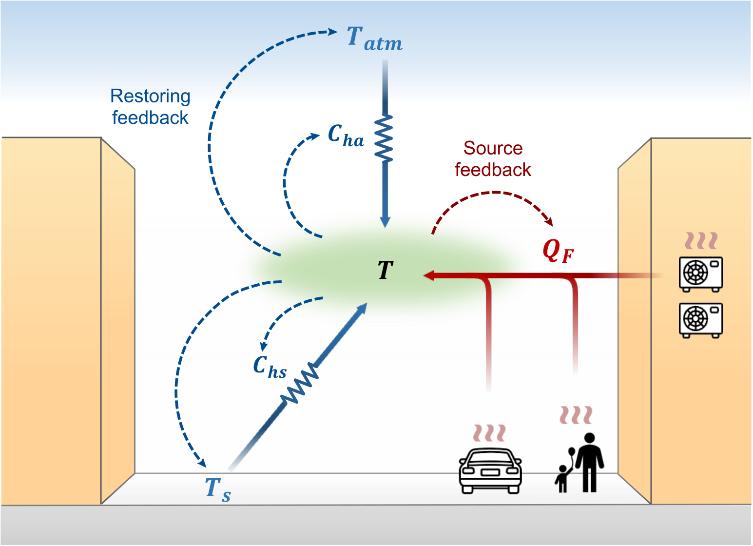
A forcing–response–feedback framework
The energy balance model (Eq. (4)) can be treated in two different ways depending on whether feedbacks are included or not. In the reference case, \(Q_{F}\) is a prescribed forcing and the parameters in the energy balance model (e.g., \(\lambda\) and \(c\)) do not depend on \(T\). When feedbacks are included, the temperature response modifies either the forcing itself or the heat-loss mechanisms.
Reference sensitivity
The simplest solution and interpretation of Eq. (4) is obtained by neglecting feedbacks and treating \(Q_{F}\), \(C\), \(\lambda\) and \(c\) as constants and thus independent of \(T\). In this case, Eq. (4) has an analytical solution \[\begin{equation} T(t)=T_{eq}+\left[T(0)-T_{eq}\right]\exp\left(-\frac{t}{\tau}\right), \end{equation}\] where \[\begin{equation} T_{eq}=\frac{Q_{F}-c}{\lambda} \tag{8} \end{equation}\] is the equilibrium temperature and \[\begin{equation} \tau=\frac{C}{\lambda} \end{equation}\] is the adjustment timescale. \(T(0)\) is the initial canopy air temperature at \(t = 0\). In this case, the temperature does not increase indefinitely, but instead relaxes exponentially toward \(T_{eq}\) with the adjustment timescale \(\tau\). One can now see that \(C\) represents the thermal inertia of the urban canopy air layer and sets the adjustment timescale of the system. A quick estimate of \(\tau\) suggests that it is on the order of 100–1000 s for an urban canyon, corroborated by simulations in Mei and Yuan (2021). This short timescale is partly why weather and climate models tend to assume equilibrium for the canopy air energy balance (i.e., completely ignoring the effect of \(C\)).
In the following, we will only focus on the equilibrium sensitivity and thus drop the subscript ‘eq’ in the definition of anthropogenic heat sensitivity \(S\). It follows from Eq. (8) that \(\Delta Q_{F}\) produces a corresponding equilibrium temperature change of \(\Delta T =\Delta Q_{F}/ \lambda\). The anthropogenic heat sensitivity is therefore \[\begin{equation} S_0 \equiv \left.\frac{\Delta T}{\Delta Q_{F}}\right|_{ref} = \frac{1}{\lambda_0}. \tag{9} \end{equation}\] Following the terminology from the global climate change literature, we refer to \(S_0\) the reference sensitivity, where the subscript zero emphasizes that no other parameters in the system are allowed to vary with \(T\). Under these conditions, the only effect of \(\Delta Q_{F}\) is to increase \(T\) until the temperature-dependent heat-loss change (\(-\lambda \Delta T\)) balances the imposed forcing perturbation.
If \(Q_{other}\) is represented using bulk-transfer formulations (Eq. (5)), then \(\lambda = \rho c_p (C_{ha} + C_{hs})\) is controlled primarily by the efficiency of canopy air–surface and canopy air–overlying atmosphere heat exchange (Eq. (6)). Using representative values of \(\rho \sim 1\) kg m\(^{-3}\), \(c_p \sim 10^3\) J kg\(^{-1}\) K\(^{-1}\), and \(C_{ha} + C_{hs} \sim 0.1\) m s\(^{-1}\), \(\lambda\) is on the order of \(100\) W m\(^{-2}\) K\(^{-1}\). This implies a reference sensitivity on the order of \(0.01\) K (W m\(^{-2}\))\(^{-1}\), consistent with the typical magnitude of sensitivity reported in the literature (L. Wang et al. 2023). This also provides a simple explanation for the reported diurnal and seasonal variations in anthropogenic heat sensitivity (L. Wang et al. 2023). Because turbulent exchanges are generally stronger during daytime and summer conditions, \(\lambda\) tends to increase during these periods, thereby reducing anthropogenic heat sensitivity. Conversely, nighttime and wintertime conditions are associated with smaller \(\lambda\) values and therefore enhanced anthropogenic heat sensitivity. This further explains why anthropogenic heat sensitivity is typically stronger under calmer and more weakly ventilated conditions (L. Wang et al. 2023).
Previous studies that formulated canopy air heat budgets could derive a similar reference sensitivity under comparable assumptions. However, these studies did not always explicitly isolate or report this quantity, and even if they had, the exact analytical expressions would differ because the canopy air heat budget was formulated differently, particularly with respect to horizontal advection and canopy air–surface heat exchange (Xue et al. 2020; Yuan et al. 2020; Mei and Yuan 2021). These studies generally diagnose temperature responses through numerical simulations rather than analytically separating the reference sensitivity from feedbacks, which are discussed below.
Climate feedback parameters
The reference case assumes fixed anthropogenic heat flux as forcing and fixed heat-loss parameters (i.e., \(\lambda\) and \(c\)), while retaining the baseline restoring mechanism. In reality, feedbacks may arise through modifications to either the atmospheric response to the forcing or the forcing itself. Here, we distinguish between these two classes of feedbacks. The first class, termed restoring feedback, modifies the anthropogenic heat sensitivity by altering the way heat is removed from the urban canopy air. Such feedbacks emerge when \(\lambda\) and \(c\) depend on temperature, for example through changes in turbulent transport. The second class consists of feedbacks that act directly on the anthropogenic heat flux itself, termed source feedback. For example, higher outdoor temperatures can increase cooling energy demand and the associated anthropogenic heat release during summer.
These feedbacks can be incorporated into the energy balance framework by allowing both the anthropogenic heat forcing and the heat-loss parameters to depend on temperature. Let \((T_0, Q_{F,0})\) denote an equilibrium state of Eq. ((4)), so that \(Q_{F,0} = \lambda_0\, T_0 + c_0\), where \(Q_{F,0} = Q_{F}(T_0)\), \(\lambda_0= \lambda(T_0)\), \(c_0= c(T_0)\). Consider a small perturbation to the temperature-independent/background component of anthropogenic heat flux, denoted as \(\Delta Q_{F,0}\), causing a small temperature perturbation \(\Delta T\), and linearise each \(T\)-dependent quantity around \(T_0\): \[\begin{equation} Q_{F}(T) \approx Q_{F,0} + \lambda_\text{source}\, \Delta T + \Delta Q_{F,0} , \qquad \lambda(T) \approx \lambda_0 + \lambda'\, \Delta T, \qquad c(T) \approx c_0 + c'\, \Delta T, \tag{10} \end{equation}\] where \(\lambda_\text{source} \equiv \left.\partial Q_{F}/\partial T\right|_{T_0}\) is the partial derivative of \(Q_{F}\) with respect to \(T\) at \(T_0\) (units W m\(^{-2}\) K\(^{-1}\)), and \(\lambda' \equiv \left.\partial \lambda/\partial T\right|_{T_0}\) and \(c' \equiv \left.\partial c/\partial T\right|_{T_0}\) are the partial derivatives of \(\lambda\) and \(c\) with respect to \(T\) at \(T_0\), respectively. Note that the total change in anthropogenic heat flux between the two equilibrium states (i.e., \(Q_{F}(T) - Q_{F,0}\)) includes the imposed forcing (\(\Delta Q_{F,0}\)) and the source-feedback contribution (\(\lambda_\text{source}\, \Delta T\)). Substituting into Eq. ((4)), using the equilibrium condition at \(T_0\), and discarding terms quadratic in \(\Delta T\), the following anthropogenic heat sensitivity can be obtained \[\begin{equation} S_f \equiv \frac{\Delta T}{\Delta Q_{F,0}} = -\frac{1}{\Lambda}. \tag{11} \end{equation}\] where \[\begin{equation} \Lambda = \underbrace{(-\lambda_0)}_{\text{baseline}} \;+\; \underbrace{\lambda_\text{restoring}}_{\substack{\text{restoring}\\\text{feedback}}} \;+\; \underbrace{\lambda_\text{source}.}_{\substack{\text{source}\\\text{ feedback}}} \tag{12} \end{equation}\] Here, \(\lambda_\text{restoring}= -\lambda' T_0-c'\). For \(S\), a subscript ‘\(f\)’ is added to emphasize that this anthropogenic heat sensitivity parameter is defined with respect to an imposed forcing (\(\Delta Q_{F,0}\)), termed forcing-based sensitivity hereafter.
In climate feedback terminology, each term on the right-hand side of Eq. (12) may be interpreted as a climate feedback parameter and \(\Lambda\) as the total feedback parameter with units of W m\(^{-2}\) K\(^{-1}\). Eqs. (11) and (12) are written in a way that the sign of each feedback parameter in Eq. (12) directly indicates the nature of the feedback: positive values correspond to positive feedbacks that amplify the baseline temperature response, whereas negative values correspond to negative feedbacks that damp it.
Similar to the convention of referring to the Planck response as the Planck feedback in global climate feedback analysis, we refer to \((-\lambda_0)\) as the baseline feedback parameter, although it represents the intrinsic restoring tendency of the system to remove heat from the urban canopy air layer rather than a formal feedback induced by changes in the system state. It is therefore negative by design. The remaining feedback parameters quantify feedback-induced modifications to this baseline restoring tendency. A canonical example of positive feedback arises from summer air-conditioning demand, for which \(\lambda_\text{source}>0\) because cooling energy consumption and the associated anthropogenic heat increase with outdoor temperature. In contrast, a canonical example of negative feedback occurs when heat-loss processes become more efficient as the canopy air temperature increases, as may occur for positive \(\lambda’\) through enhanced turbulent transport under increasingly unstable stratification.
Two limiting cases are worth noting. When all feedback parameters vanish, \(\Lambda=-\lambda_0\) and the reference sensitivity in Eq. ((9)) is recovered. On the other hand, as the positive feedback increasingly offsets the negative baseline restoring, \(\Lambda\) approaches zero and the sensitivity is greatly amplified. Such high-sensitivity regimes may emerge during heatwaves or weakly ventilated nighttime conditions in dense urban environments with strong air-conditioning feedbacks.
Before closing this section, it is useful to define an effective sensitivity based on the total realized change in anthropogenic heat flux, \(Q_F(T)-Q_{F,0}\), which again includes both the forcing component (\(\Delta Q_{F,0}\)) and the source-feedback contribution (\(\lambda_\text{source}\, \Delta T\)), as follows: \[\begin{equation} S_{e} \equiv \frac{\Delta T}{Q_{F}(T)-Q_{F,0}}. \tag{13} \end{equation}\] This definition is particularly relevant when the forcing component cannot be cleanly separated from source-feedback contribution (e.g., when part or all of anthropogenic heat fluxes are generated interactively). Under such conditions, the diagnosed sensitivity usually corresponds to the effective anthropogenic heat sensitivity \(S_e\). Recovering \(S_f\) requires estimating the anthropogenic heat flux that would occur in the absence of source feedback. However, there is no generally accepted approach for constructing this counterfactual estimate at present, and some implementations may raise energy-conservation concerns (Kikegawa et al. 2022). Throughout this review, forcing-based sensitivities (\(S_f\)) and effective sensitivities (\(S_e\)) are therefore distinguished whenever possible.
Interpreting the forcing–response–feedback framework
Source feedback and gain factor.
The present framework recovers earlier gain-factor formulations (Ginzburg and Demchenko 2017, 2019; Kikegawa et al. 2022) that have been used to describe source feedback associated with building energy consumption. Within the present notation and without considering restoring feedback (i.e., \(\lambda' = c' =0\)), the temperature response reduces to \(\Delta T = \Delta T_0/(1-g_A)\), where \(\Delta T_0=S_0\Delta Q_{F,0}\) is the reference or baseline temperature response, and \(g_A \equiv \lambda_\text{source} S_0 \equiv \lambda_\text{source} /\lambda_0\) is the gain factor associated with source feedback, which determines the amplification of the reference temperature response arising from temperature-dependent anthropogenic heat flux. Hence, the present framework generalizes these earlier gain-factor formulations by incorporating both source and restoring feedbacks in a unified manner.
Restoring feedback decomposition.
The separation of \(\lambda_\text{restoring}\) into the two terms involving \(\lambda'\) and \(c'\) is unique to the linear model for \(Q_{other}\), which is adopted here for illustrative purposes. Alternative decompositions of the total restoring feedback are possible. For example, using Eqs. (6) and (7), L. Wang et al. (2023) decomposed their restoring feedback in terms of conductance feedbacks and temperature feedbacks, rather than \(\lambda'\) and \(c'\) feedbacks. More subtly, a shift in the temperature origin can redistribute part of the total restoring feedback between the \(\lambda'\) and \(c'\) terms. Consequently, the physically meaningful quantity is the total restoring feedback \(\lambda_\text{restoring}\).
Further generalization
When \(Q_{other}\) is not represented by a linear model or when it includes processes other than those considered here, the baseline feedback parameter can be interpreted as the local sensitivity of \(Q_{other}\) to canopy air temperature, \(\partial Q_{other}/\partial T\), evaluated at the reference state and with other variables held fixed. The restoring feedback is then given by the difference between the total temperature derivative and this baseline restoring, \(\lambda_\text{restoring}={dQ_{other}}/{dT}-{\partial Q_{other}}/{\partial T}\). With the linear model adopted here, these expressions reduce to \(\partial Q_{other}/\partial T = -\lambda_0\) and \(\lambda_\text{restoring}=-\lambda'T_0-c'\), respectively, consistent with the derivations presented earlier.
Although the present review has focused on the canopy air heat budget, the same forcing–sensitivity–feedback framework can be applied to other temperature variables and control volumes governed by different energy budgets. For example, Khanh et al. (2025) treated the urban boundary layer as a well-mixed control volume and assumed that outgoing longwave radiation is the only explicit heat-loss mechanism (i.e., \(Q_{\mathrm{other}}=-\varepsilon\sigma T^4\)), where \(\varepsilon\) is the atmospheric emissivity, \(\sigma\) is the Stefan–Boltzmann constant, and \(T\) is the boundary-layer temperature. At equilibrium, linearizing the emitted longwave radiation about a reference state yields a baseline feedback parameter of \({\partial Q_{\mathrm{other}}}/{\partial T}=-4\varepsilon\sigma T_0^3\) and a corresponding baseline sensitivity of \((4\varepsilon\sigma T_0^3)^{-1}\). This example illustrates that the analytical expressions for the baseline sensitivity and feedback parameters depend on the selected control volume and the heat-loss mechanisms included in its energy budget, whereas the underlying forcing–sensitivity–feedback framework remains unchanged.
This formalism provides the organizing principle for the remainder of the review. Section 3 examines \(Q_F\) broadly as an urban climate forcing. Although the theoretical framework developed here distinguishes imposed forcing from source feedback, Section 3 does not separate these contributions, but instead focuses on the magnitude, spatial and temporal variability, scale dependence, global representation, and uncertainty of \(Q_F\) as a heat input to the urban climate system. Section Sensitivity examines the anthropogenic heat sensitivity by synthesizing reported \(S_f\) and \(S_e\) across observations and numerical models. Section Feedback examines the restoring and source feedbacks that modulate urban temperature responses.
Forcing
Early reviews established the foundational methods for estimating \(Q_F\), including energy-consumption inventories, residual surface energy balance approaches, and BEMs (Sailor 2011). More recent reviews have synthesized the expanding literature on \(Q_F\) estimation, including the advances and challenges associated with these foundational methods, as well as the growing use of remote sensing data and machine learning techniques (Lu et al. 2024; Feng et al. 2025). Building on these syntheses, this section focuses on what recent studies reveal about anthropogenic heat as an urban climate forcing, with particular attention to its magnitude, spatiotemporal variability, scale dependence, and uncertainty.
From bulk estimates to structured forcing
The variability and scale dependence of \(Q_F\) have long been recognized (see e.g., SMIC 1971). The global, annual mean \(Q_F\) is generally on the order of \(0.01\) W m\(^{-2}\). However, this aggregation masks its strong concentration in urban cores, industrial districts, transport corridors, and dense building clusters; it also obscures strong diurnal, weekly, seasonal, and weather-related variability associated with commuting, occupancy, appliance use, heating, ventilation, and air conditioning (HVAC) operation. At finer spatial and temporal scales, reported values can be several orders of magnitude larger. For example, the estimated peak \(Q_F\) values of 1590 W m\(^{-2}\) in central Tokyo during winter (Ichinose et al. 1999), and up to 6000 W m\(^{-2}\) for data centers in Phoenix, Arizona (Sailor et al. 2026), are among the highest reported in the literature. Recent advances in estimating \(Q_F\) can be broadly viewed as efforts to characterize it as a spatially heterogeneous, temporally variable, and sectorally structured urban climate forcing.
Spatial heterogeneity
Earlier inventories often disaggregated energy statistics using population or land-use proxies, whereas more recent studies increasingly combine geospatial analysis techniques with remote sensing products to better resolve intra-urban heterogeneity. Among these developments, satellite-based residual surface energy balance approaches using multispectral sensors (e.g., Landsat) have been applied to estimate spatially varying \(Q_F\) over Fuzhou (Zhang et al. 2012), Delhi (Chakraborty et al. 2015), Athens and Paris (Bliziotis et al. 2017), and a variety of urban environments (Bala et al. 2024). In these approaches, \(Q_F\) is estimated as the residual of the urban surface energy balance equation (i.e., Eq. (1)), so uncertainties in the estimated radiative, sensible, latent, and ground heat fluxes propagate directly into the inferred anthropogenic heat flux. In addition, because the estimates are usually tied to clear-sky satellite overpasses, they provide only snapshots in time and cannot resolve the full diurnal cycle or variability associated with changing weather conditions (Chrysoulakis et al. 2018; Bala et al. 2024).
A range of remote sensing products has been used to spatially resolve \(Q_F\), including nighttime light data (B. Chen et al. 2016; Lin and Xu 2020), active fire data for detecting heavy emissions from industrial plants (Zhang et al. 2019), and ground- or satellite-based pollutant emissions records (Lee et al. 2014). As discussed further in Section Global datasets, global datasets have increasingly adopted data-fusion approaches that combine satellite products with sociodemographic information (Rashinkar and Krushnasamy 2017). Machine-learning techniques, such as cubist and random forest algorithms, have further extended this line of research (Chen et al. 2020; Ao et al. 2024; He et al. 2023; Lin and Xu 2020). These developments have substantially improved the spatial detail of \(Q_F\) estimates, but they also introduce uncertainties associated with the selection, quality, representativeness, and transferability of the predictors used to spatially disaggregate \(Q_F\).
Temporal variability
The temporal variability of \(Q_F\) has long been recognized, with diurnal, weekly, and seasonal cycles reflecting traffic activity, weekday–weekend differences, occupancy patterns, and heating and cooling demand (Oke et al. 2017). Beyond these established patterns, two critical temporal dynamics remain poorly understood: (1) short-term lags between building energy consumption and anthropogenic heat release, and (2) long-term changes in both past and future anthropogenic heat fluxes.
Building energy consumption and anthropogenic heat release are not always temporally coincident because of thermal storage. At the building scale, Liu et al. (2022) showed that the hourly ratio of actual anthropogenic heat release to electricity consumption can vary from negative values to well above unity. At the city scale, Yu et al. (2021) demonstrated that neglecting thermal storage can distort the disaggregation of \(Q_F\) based on local climate zones, yet this effect has not been considered in many datasets.
At longer time scales, studies have estimated long-term increases in global \(Q_{F}\) through past, middle, and late twenty-first century (Lu et al. 2017; Jin et al. 2019; Varquez et al. 2021). Regional to local scenario studies increasingly examine how development pathways, building efficiency, air-conditioning adoption, and transportation electrification alter future \(Q_F\) (Darmanto et al. 2019; Ribeiro et al. 2021). These projections, which are designed to be consistent with integrated climate change scenarios (e.g., Representative Concentration Pathways, Shared Socioeconomic Pathways), emphasize that future \(Q_F\) estimates should not be inferred from population growth alone, but also from changes in background climate, cooling/heating demand, technological advancements influencing energy use efficiency, and other socioeconomic factors.
Sector-specific forcing
Another recent development is the increasingly explicit representation of sector-specific anthropogenic heat fluxes. BEMs coupled with urban land surface and atmospheric models have enabled dynamic estimates of anthropogenic heat fluxes from the building sector under different climate, retrofit, and urban development scenarios (Crawley et al. 2001; Singh, Mughal, et al. 2022). Transportation has evolved from simple traffic-volume-based estimates toward trajectory-resolved and model-integrated representations, allowing assessment of emerging technologies such as vehicle electrification (Ivanchev et al. 2020; Mussetti et al. 2022; Chen and Yang 2022; Hata et al. 2025; Cao et al. 2022; Colas et al. 2025; Sun et al. 2026). Recent studies have also begun to isolate high-intensity point sources, including industrial facilities and data centers (Sailor et al. 2026), which may contribute little to city-wide averages but can generate substantial localized heat emissions (Lee 1979; Baniata et al. 2021; Singh, Bhati, et al. 2022; Varquez et al. 2021).
Sector-specific estimates have improved the partitioning of \(Q_F\) among buildings, transportation, industry, and other sources. However, partitioning by sector is not the same as representing the forcing pathway. For example, \(Q_F\) released at street level by vehicles, ejected from HVAC systems at varying building facades, or emitted from industrial stacks can interact with the urban climate system in fundamentally different ways. This makes source-pathway representation a major unresolved challenge in anthropogenic heat research.
Global datasets
| Dataset | Spatial Resolution | Period | Temporal Resolution | Methodology | Sectoral Decomposition | Reported \(Q_F\) statistics | ||
|---|---|---|---|---|---|---|---|---|
| 7-9 | Averaging Basis | Mean \(Q_F\) (\(\mathrm{W\,m^{-2}}\)) | Max \(Q_F\) (\(\mathrm{W\,m^{-2}}\)) | |||||
| Flanner2009 (Flanner 2009) | 0.5\(^\circ\) (finest) | 2005, 2040, 2100 | Hourly, seasonal | Disaggregation of national energy statistics via population density; diurnal weightings and latitude-sinusoid temporal profiles | Aggregate energy use | Whole Earth | 0.028 (2005); 0.059 (2040); 0.19 (2100) | 48 (New York, \(0.5^\circ\) resolution) |
| LUCY (Allen et al. 2011) | 2.5 arc-min | Contemporary | Hourly | Sectoral disaggregation (buildings, transport, metabolism) with country-specific work schedules and degree-day climatology | Buildings, transport, metabolism | Urban | 0.7–3.6 (typical urban daytime min and max) | 577 (New York); 262 (Paris); 178 (Tokyo) |
| Chen and Shi (2012) (Chen and Shi 2012) | 30 arc-sec | 2006 | Annual | DMSP/OLS nighttime lights calibrated with state-level energy statistics | Aggregate energy use | Land surface | 0.10 | \(>\)100 |
| Dong et al. (2017) (Dong et al. 2017) | 30 arc-sec | Contemporary | Hourly | Sectoral disaggregation of energy statistics using population density, nighttime lights, empirical temperature-energy relations, and temporal templates | Buildings, industry, transport, metabolism | Land surface | 0.13 | 493 (Hong Kong); 353 (Singapore) |
| AH-DMSP (2017) (Yang et al. 2017) | 1 km | 1992–2010 | Annual | Statistical modeling (nighttime lights, NDVI, population, EIA statistics) of long-term annual trends | Aggregate energy use | Not reported | Not reported | 581.3 (unspecified grid) |
| PF-AHF (2019) (Jin et al. 2019) | 30 arc-sec | 1970–2050 | Annual | Population-density disaggregation of BP energy statistics | Aggregate energy use | Land surface | 0.05 (1970); 0.13 (2015); 0.16 (2050) | Not reported |
| AH4GUC (Varquez et al. 2021) | 1 km | 2010s, 2050s | Hourly | Extension of Dong et al. (2017) incorporating VIIRS datasets and future projections | Buildings, industry, transport, metabolism | Whole Earth | 0.031 (2010s); 0.050 (2050s) | Not reported |
| Wang et al. (2022) (Wang et al. 2022) | 500 m | 2016 | Monthly | Multi-source data fusion with local temperature degree-day scaling | Building, industry, transport, metabolism | Land surface | 0.19 | 438 (London); 406.4 (New York); 356.5 (Tokyo) |
Notes. Temporal coverage refers to the years represented by each dataset, whereas temporal resolution denotes the frequency at which anthropogenic heat fluxes are reported. Mean \(Q_F\) values are reported using different spatial averaging operators (whole Earth, land surface, or urban areas) and are therefore not directly comparable. Max \(Q_F\) values correspond to the largest values explicitly reported in each study and may represent regional means, grid-cell maxima, or threshold values.
Sailor (2011) concluded by calling for standardized anthropogenic heat flux products for atmospheric modeling, analogous to global land-use and land-cover forcing datasets. Over the past decade, this vision has largely been realized through several global and continental-scale datasets that now provide \(Q_F\) forcing for regional and global climate models. These datasets have greatly expanded the accessibility of \(Q_F\) information, particularly for data-sparse regions, and enabled systematic intercomparison across cities and climate zones.
Table 1 highlights eight such datasets, revealing a clear trend toward increasingly resolved representation of \(Q_F\). Spatial resolution has improved from 0.5\(^\circ\) to 500 m, allowing increasingly detailed depiction of urban hotspots. Temporal representation has likewise evolved from annual means, to resolving seasonal and daily variations, and to hourly estimates incorporating sector-specific and weather-dependent temporal profiles. At the same time, methodologies have progressed from simple population-based disaggregation of national energy statistics toward increasingly sophisticated approaches that incorporate nighttime lights, sector-specific information, and, more recently, multi-source data fusion. However, the increased realism does not necessarily imply reduced uncertainty. Differences in spatial resolution, temporal representation, source allocation, and downscaling strategy can produce substantially different \(Q_F\) estimates. Consequently, although most datasets reproduce similar large-scale geographical patterns, they can diverge markedly in the magnitude and distribution of \(Q_F\) within individual cities.
Figure 2 illustrates these uncertainties by comparing several global datasets over Kinshasa, London, and Singapore. Kinshasa provides a useful test case because it is a rapidly growing tropical megacity with limited local urban climate observations. In such a data-sparse region, global datasets can provide a first approximation of anthropogenic heat forcing, but they also reveal substantial differences: the Flanner2009 dataset produces an empty field over Kinshasa (and uniform values in the other two cities) owing to its coarse resolution, whereas finer resolutions mainly disagree according to the treatment of spatial disaggregation: from purely relying on nighttime lights products (Yang et al. 2017), population datasets (Jin et al. 2019) or a combination of both (Dong et al. 2017; Varquez et al. 2021). While verifications have been conducted for these datasets, through comparisons with either other \(Q_{F}\) proxies such as nighttime lights (Jin et al. 2019) or bottom-up estimates (Dong et al. 2017; Varquez et al. 2021) including power-plant locations (Varquez et al. 2021), their spatial contrasts serve as a reminder that these global datasets are not direct observations of \(Q_F\); they are estimates that encode assumptions about where human activity, energy use, and anthropogenic heat are located.
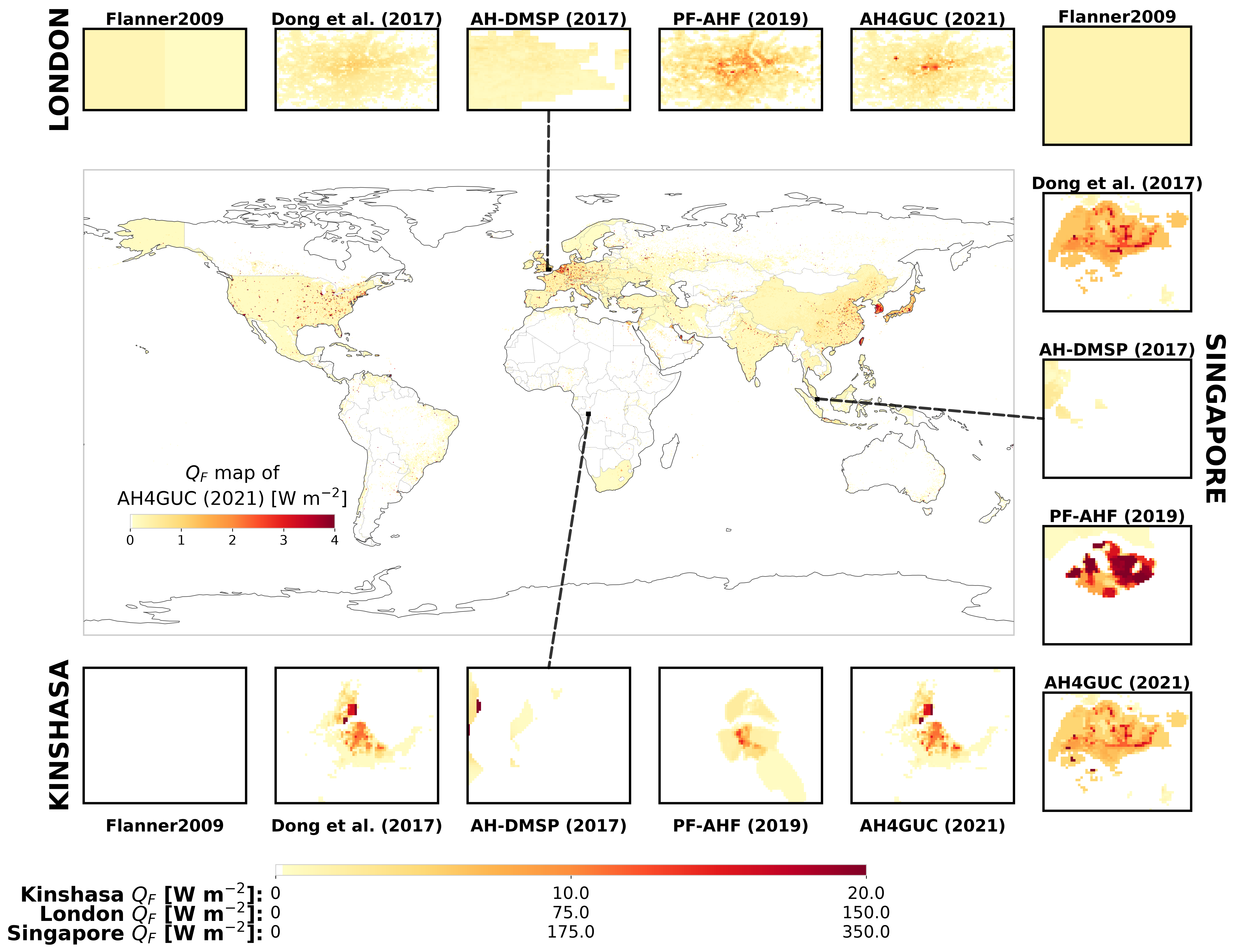
The comparison for London and Singapore further demonstrates that global datasets tend to agree more closely in their city-scale averages than in their representation of localized hotspots. For London, local top-down and bottom-up inventories estimate annual mean \(Q_F\) values of approximately 5.79–10.9 W m\(^{-2}\), with central London reaching 57.5–123.5 W m\(^{-2}\) (Capel-Timms et al. 2020; Iamarino et al. 2011; Harrison et al. 1984). Modeling studies suggest even higher peak daytime values exceeding 300 W m\(^{-2}\) in WRF-SUEWS simulations (Sun et al. 2024). The global datasets produce city-mean values broadly consistent with this range, but differ substantially in their representation of hotspots.
For Singapore, the discrepancy is even larger than for London. The global datasets exhibit a wider spread in both city-scale means and local pixel values: some products produce low urban-core values, whereas others generate very large industrial maxima, particularly when point-source information such as Visible Infrared Imaging Radiometer Suite Nightfire is incorporated (Varquez et al. 2021). Local building inventories estimate a building-only city-wide mean of approximately 10.1 W m\(^{-2}\) and a commercial peak of 663 W m\(^{-2}\) (He et al. 2023), while bottom-up inventories (Quah and Roth 2012), transport mobility modeling (Ivanchev et al. 2020), and coupled mesoscale simulations (Singh, Mughal, et al. 2022) indicate non-negligible traffic contributions. This comparison suggests that compact and industrially heterogeneous cities pose particular challenges for global datasets.
Overall, the global dataset comparison highlights two major sources of uncertainty. The first is spatial smoothing: coarse grids dilute compact urban cores, transport corridors, and high-emitting industrial zones. The second is proxy sensitivity: assumptions about spatial allocation can produce substantially different \(Q_F\) fields even when aggregate energy consumption is similar. These uncertainties do not invalidate the usability of global datasets, which are indispensable for climate modeling and for regions lacking local inventories. However, they should be interpreted as scale-dependent forcing estimates rather than direct observations of \(Q_F\).
The studies reviewed in this section suggest that our ability to characterize anthropogenic heat as an urban climate forcing has substantially advanced, revealing its strong spatial heterogeneity, temporal variability, sectoral breakdowns, and scale dependence. However, the magnitude and representation of the forcing alone do not determine its climatic significance. The same anthropogenic heat flux can produce markedly different temperature responses depending on the characteristics of the urban environment and the way \(Q_F\) is introduced into the urban climate system. Quantifying these responses therefore requires moving beyond examining the forcing itself to investigating the sensitivity of urban temperatures to anthropogenic heat flux, which is the focus of the next section.
Sensitivity
Anthropogenic heat sensitivity quantifies the temperature response associated with a unit change in anthropogenic heat flux. Available estimates are derived from both observations and numerical simulations. Here, we classify a study as observational or numerical according to whether the temperature response is measured or simulated; an observational estimate may therefore still rely on model-derived estimates of anthropogenic heat flux.
Observational estimates remain relatively uncommon because isolating the temperature response to anthropogenic heat flux from concurrent variations in meteorological conditions, land cover, and other urban processes is inherently difficult. Studies that successfully constrain anthropogenic heat sensitivity using observations are therefore particularly valuable and are discussed first below, followed by the much larger body of numerical modeling studies. In numerical experiments, anthropogenic heat flux may either be prescribed or generated interactively by a coupled BEM or another model component. As discussed in Section Theory, prescribed-forcing experiments yield forcing-based sensitivity (\(S_f\)), whereas coupled simulations generally yield effective sensitivity (\(S_e\)), unless the total anthropogenic heat flux change can be separated into forcing and source-feedback contributions. Observational estimates generally face the same decomposition problem and are therefore more comparable to \(S_e\) than to \(S_f\).
Observational studies
Observational studies on the climatic effects of anthropogenic heat flux, or more broadly urbanization, generally exploit natural temporal or spatial variations in human activity, following the conceptual framework articulated by Lowry (1977). Temporal variations, such as weekday–weekend contrasts (Mitchell 1953; Kikegawa et al. 2014) or larger disruptions like G20 summit and COVID-19 lockdown (Pal et al. 2021; Meng et al. 2023), provide “natural experiments’’ in which changes in anthropogenic activity induce corresponding changes in urban temperature. These “natural experiments’’ have also been studied numerically (e.g., Kikegawa et al. 2014, 2022; Nakajima et al. 2021; Takane et al. 2022). Other studies instead examine spatial co-variations between anthropogenic activity indicators and urban temperatures or UHI intensities using dense station networks or remote sensing products (He et al. 2020; Jin et al. 2020; Zhu et al. 2017).
Two principal challenges arise when interpreting these studies. First, observational studies rarely quantify the anthropogenic heat flux change (\(\Delta Q_F\)) associated with the observed temperature response (\(\Delta T\)). Second, even when \(\Delta Q_F\) is estimated, observed temperature variations reflect the combined influence of meteorological variability, land-cover heterogeneity, topography, and other urban processes. Consequently, it is generally difficult to attribute observed \(\Delta T\) uniquely to the effect of anthropogenic heat flux.
To address these challenges, particularly the second, studies have adopted statistical approaches designed to reduce the influence of co-varying processes, including stepwise multiple linear regression models (Y. Chen et al. 2023), partial least squares regression models (Chen, Wang, Zhou, et al. 2025), linear mixed-effects models (Qian et al. 2023), and machine-learning methods such as random forest (Chen, Wang, Luo, et al. 2025) and Light Gradient Boosting Machine (Sheng et al. 2025). Nevertheless, interpreting the results using anthropogenic heat sensitivity remains challenging. First, the reported results are not always directly comparable to the anthropogenic heat sensitivity defined in the present review. For example, some studies report standardized regression coefficients (e.g., Qian et al. 2023; Chen, Wang, Luo, et al. 2025), whereas others stratify the temperature response into different UHI categories (e.g., Sheng et al. 2025), making it difficult to translate the results into physically interpretable sensitivities with units of K (W m\(^{-2}\))\(^{-1}\). Second, the inferred relationships sometimes appear physically counterintuitive. For example, some models yield negative coefficients during certain periods or for certain anthropogenic heat flux components (e.g., Y. Chen et al. 2023; Chen, Wang, Zhou, et al. 2025), despite the expectation that anthropogenic heat flux should generally induce warming effects. Likewise, although anthropogenic heat flux effects are expected to be stronger at night and during winter, some studies identify anthropogenic heat flux variables only in summer prediction equations but not in winter equations (e.g., see Table 2 of Y. Chen et al. 2023) or only for daytime but not for nighttime (see Table 4 of Chen, Wang, Zhou, et al. 2025). These examples illustrate that anthropogenic heat sensitivities inferred statistically from observational data depend not only on the underlying physical relationship but also on the statistical model formulation, including the choice of predictors, variable transformations, spatial and temporal aggregation, and treatment of co-varying factors.
Another approach exploits both spatial and temporal contrasts in human activity through a difference-in-differences framework. For example, Kikegawa et al. (2014) compared weekday–weekend temperature contrasts between commercial and residential districts. The temporal contrast reflects changes associated with reduced human activity during weekends, while the spatial contrast between commercial and residential areas helps remove background meteorological variability affecting both locations. Electricity demand was used as a proxy for anthropogenic heat flux. This approach yielded afternoon sensitivities of approximately 0.01 K (W m\(^{-2}\))\(^{-1}\) for both Osaka and Tokyo, Japan. The sensitivity estimated by Kikegawa et al. (2014) is notable because, as shown in the following section, it falls within the range commonly reported in numerical modeling studies, thereby providing one of the clearest observational benchmarks for anthropogenic heat sensitivity. Similarly, Ohashi et al. (2016) examined seasonal variations in weekday–weekend temperature contrasts across multiple urban districts in Osaka, Japan, and related them to seasonal differences in electricity consumption. However, their temperature response and electricity-consumption change were evaluated over different time periods, making the resulting ratio difficult to interpret. This example motivates the temporal and spatial consistency criteria introduced in the following subsection for synthesizing anthropogenic heat sensitivities from numerical studies.
Numerical studies
Numerical studies of anthropogenic heat flux effects have evolved alongside the development of urban climate models. Early studies primarily used bulk surface energy balance models, either in offline mode or coupled to one-, two-, and three-dimensional atmospheric models. Beginning around the 2000s, urban canopy models (UCMs) introduced more explicit representations of urban geometry and canopy air energy exchange, and have since been coupled to weather, climate, and Earth system models. Other studies have also employed computational fluid dynamics tools to resolve urban flow and transport processes at building and street-canyon scales. Because anthropogenic heat sensitivities are rarely reported explicitly in these studies, this subsection focuses on those from which forcing-based or effective sensitivities can be extracted or reasonably inferred. Rather than attempting a comprehensive survey of the numerical modeling literature, we synthesize a representative set of 44 studies across time, from which we extract 81 sensitivity estimates.
To facilitate meaningful comparisons across models, scales, and study settings, anthropogenic heat sensitivity is diagnosed only when \(\Delta T\) and \(\Delta Q_F\) are averaged over consistent temporal periods and spatial domains. For example, a daily mean temperature response is paired with a daily mean anthropogenic heat flux, whereas a domain-mean temperature response at a given hour is paired with the domain-mean anthropogenic heat flux over the same hour. In contrast to previous work that included estimates based on the ratio of a peak temperature response to a peak anthropogenic heat flux (L. Wang et al. 2023; Xie et al. 2024), such estimates are excluded from our synthesis. We nevertheless recognize that different averaging operators could, in principle, be applied to \(\Delta T\) and \(\Delta Q_F\), and discuss the challenges associated with defining appropriate temporal and spatial averaging operators in Section Future outlook. In addition, our synthesis focuses on near-surface air temperature such as the canopy air temperature and 2-m air temperature and does not consider land surface temperature.
Typical magnitude and major sources of variability in anthropogenic heat sensitivity
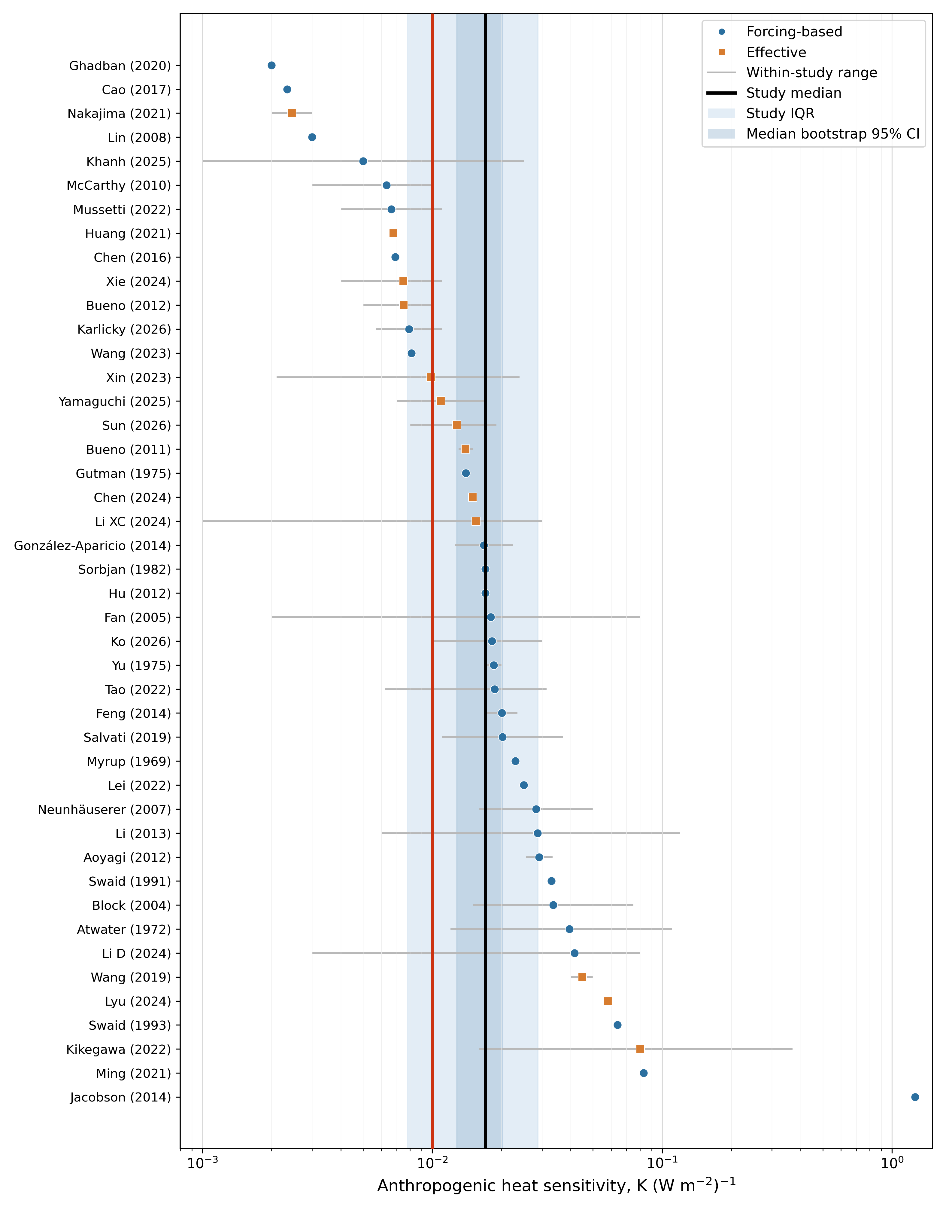
A study-level synthesis of diagnosed sensitivities shows that most reported values cluster within a relatively narrow order-of-magnitude range despite large differences in model formulations, study regions, temporal and spatial scales, and experimental design (Figure 3). The median study-level sensitivity is 0.017 K (W m\(^{-2}\))\(^{-1}\), with an interquartile range of 0.008–0.029 K (W m\(^{-2}\))\(^{-1}\). This synthesis supports a practical rule-of-thumb value of order \(0.01\) K (W m\(^{-2}\))\(^{-1}\) for quick estimates of local- to regional-scale near-surface air-temperature responses to anthropogenic heat flux. Interestingly, this value is independently constrained by the observational analysis of Kikegawa et al. (2014).
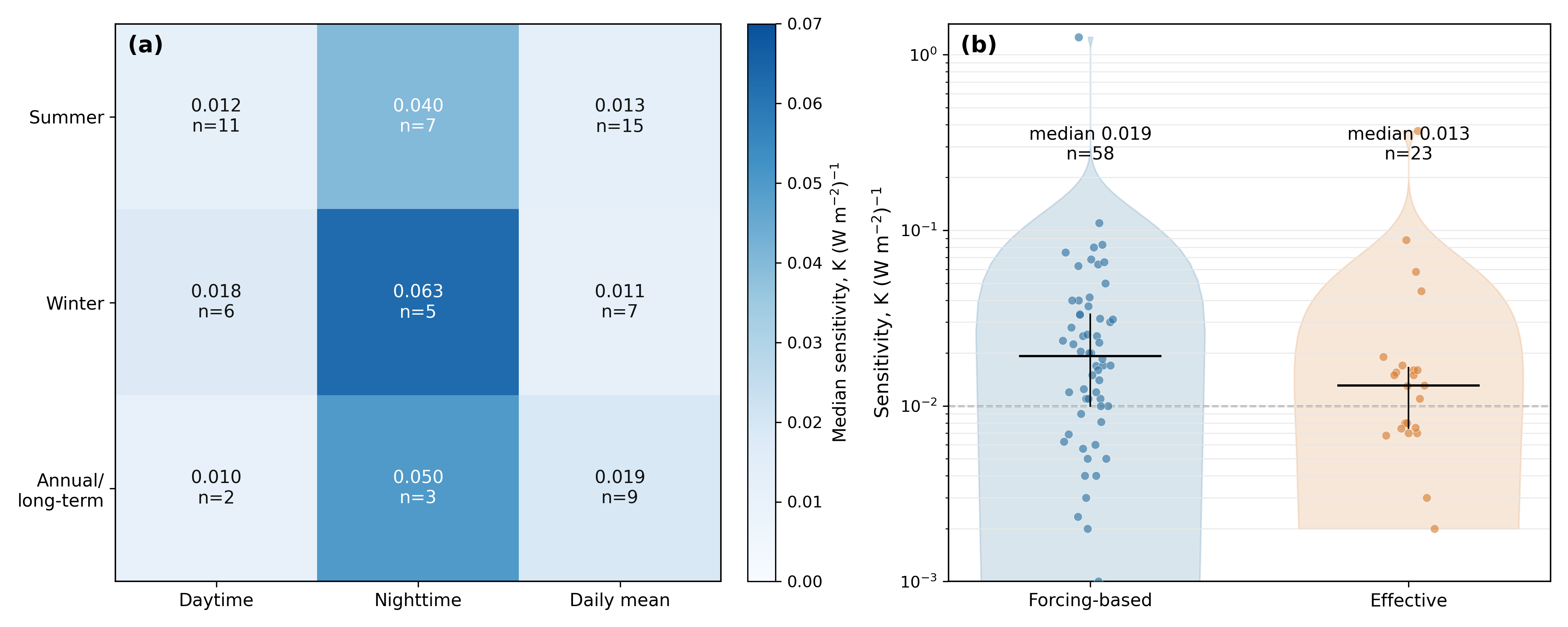
Across all the studies examined here, sensitivities tend to be larger at night than during the day, and the contrast is especially pronounced in winter (Figure 4a). In the extracted estimates, the median sensitivity increases from approximately 0.012 K (W m\(^{-2}\))\(^{-1}\) during summer daytime to 0.040 K (W m\(^{-2}\))\(^{-1}\) during summer nighttime, and from 0.018 K (W m\(^{-2}\))\(^{-1}\) during winter daytime to 0.063 K (W m\(^{-2}\))\(^{-1}\) during winter nighttime. This pattern is consistent with the physical understanding that anthropogenic heat flux warms the near-surface atmosphere more efficiently when turbulent mixing is weaker, boundary layers are shallower, and background radiative forcing is smaller.
The typical magnitude of anthropogenic heat sensitivity and its systematic day–night and summer–winter contrasts are already evident in early modeling studies. In fact, the 7 pre-2000 modeling studies included in our synthesis yield a median sensitivity that is not statistically distinguishable from that of the remaining post-2000 studies based on a permutation test, and one of the earliest studies, Atwater (1972), had already reported both day–night and summer–winter contrasts. What could not be assessed from the pre-2000 literature, because all of those studies prescribed \(Q_F\) as an external forcing, and emerges from the present synthesis is the importance of how anthropogenic heat sensitivity is defined. Forcing-based sensitivities (\(S_f\)) have a higher median value than effective sensitivities (\(S_e\)): approximately 0.019 K (W m\(^{-2}\))\(^{-1}\) for \(S_f\) compared with 0.013 K (W m\(^{-2}\))\(^{-1}\) for \(S_e\) (see Figure 4b).
At first glance, this result may appear counterintuitive. Because positive source feedbacks, which are more commonly represented in the studies reporting \(S_e\) here, amplify the temperature response to a given anthropogenic heat forcing, one might expect studies that include such feedbacks to exhibit higher, rather than lower, anthropogenic heat sensitivities. However, the result is fully consistent with the definitions of \(S_f\) and \(S_e\). The forcing-based sensitivity \(S_f\) relates the temperature response to the forcing alone, whereas the effective sensitivity \(S_e\) is defined using the total anthropogenic heat flux change, which includes both the forcing and the additional anthropogenic heat generated through source feedback. The apparent contradiction can therefore be reconciled by recognizing that, although a positive source feedback amplifies the temperature response, it simultaneously increases the diagnosed \(\Delta Q_F\) in the denominator of \(S_e\). Consequently, the lower median value of \(S_e\) does not imply a weaker thermal response, but instead reflects the different definition of anthropogenic heat sensitivity.
More broadly, this distinction emphasizes that the intuitive connection between positive feedback and increased climate sensitivity applies only to the forcing-based sensitivity \(S_f\) defined here (see Eqs. (11) and (12)), whereas the effective sensitivity \(S_e\) cannot be interpreted using the same relationship. Accordingly, studies that represent source feedback but seek to interpret their sensitivity results from a feedback perspective, to be discussed in Section Feedback, must separately define a forcing-based sensitivity. The practical challenges involved in defining such a forcing-based sensitivity are discussed further in Section Future outlook.
Methodological sources of variability in anthropogenic heat sensitivity
The synthesis above highlights that anthropogenic heat sensitivity depends on season and time of day, as well as on whether it is defined as a forcing-based or effective sensitivity. Beyond these factors, additional and more subtle sources of variability arise from methodological choices.
The first issue concerns the definition of anthropogenic heat flux itself. Although \(Q_F\) is broadly interpreted as the sensible heat released by human activities into the urban environment in this review, different studies have adopted different definitions (Liu et al. 2022; Xie et al. 2024). Traditional inventory-based approaches typically estimate \(Q_F\) from energy consumption, whereas building energy studies may define it in terms of the net heat exchanged between buildings and the outdoor urban environment, including heat transported through ventilation, infiltration, and HVAC systems (Sailor 2011). As emerging technologies such as air-source heat-pumps become more widespread, these distinctions are likely to become increasingly important. Consequently, reported anthropogenic heat sensitivities may differ simply because the underlying definition of \(Q_F\) differs.
The second issue concerns the reference area used to define \(Q_F\), which directly affects its reported magnitude (Best and Grimmond 2016). Establishing a consistent reference area is challenging because anthropogenic heat is represented differently across models. Mesoscale models, for example, often prescribe \(Q_F\) as an areal flux density, whereas computational fluid dynamics simulations (e.g., Zhang et al. 2024) and laboratory experiments (e.g., Liu et al. 2025) may prescribe anthropogenic heat as line or volumetric heat sources. Comparisons with conventional area-based definitions of \(Q_F\) are therefore less straightforward.
A related issue is that, for the diagnosed sensitivity to be physically meaningful, the reported temperature and \(Q_F\) should correspond to compatible spatial supports, such as a street canyon, urban tile, model grid cell, or observation footprint. In many models, however, they do not. For example, in the Single-Layer Urban Canopy Model (SLUCM) coupled to the Weather Research and Forecasting (WRF) model, \(Q_F\) is expressed per unit impervious urban land area, including both roofs and street canyon floors, whereas canopy air temperature represents only the air within the street canyon. The diagnosed sensitivity of canopy air temperature to \(Q_F\) therefore depends strongly on the ratio of roof area to canyon-floor area (D. Li et al. 2024). Similarly, 2-m air temperature represents the entire model grid cell, whereas \(Q_F\) is applied only over the impervious urban fraction of that grid cell. The diagnosed sensitivity based on 2-m air temperature therefore depends on the impervious urban land fraction (D. Li et al. 2024).
The third issue concerns how sensitivity is computed. Because \(\Delta T\) and \(\Delta Q_F\) are not always available over consistent spatial domains and temporal periods, estimating their ratio may require judgment in pairing the two quantities, producing a range of plausible sensitivity estimates that reflects this ambiguity. The choice of spatial and temporal averaging operators, which varies across studies in Figure 3, also plays an important role. One notable example is the sensitivity inferred from Jacobson (2014), which is approximately 1.2 K (W m\(^{-2}\))\(^{-1}\), nearly two orders of magnitude larger than the median across studies. This exceptionally large value partly reflects the small magnitude of the globally averaged \(\Delta Q_F\) and highlights the importance of considering internal variability when diagnosing the temperature response to a small forcing, as discussed below. Other studies estimate sensitivity by fitting a linear relationship between \(\Delta T\) and \(\Delta Q_F\) and interpreting the fitted slope as the sensitivity. This approach is generally less sensitive to individual outliers. However, the fitted sensitivity depends on the number, range, and distribution of the sampled data points, which are themselves influenced by the chosen spatial and temporal averaging operators. The effects of these averaging operators are discussed further in Section Future outlook.
Sources of uncertainty in anthropogenic heat sensitivity
The previous subsection focuses on methodological choices that can lead to different reported anthropogenic heat sensitivities. Here, we distinguish these methodological differences from uncertainty in the diagnosed sensitivity itself, which arises primarily from internal variability and structural uncertainty.
Because the climate system is chaotic, the simulated temperature response to anthropogenic heat flux contains both the forced signal and internally generated fluctuations. This issue is particularly important in global simulations, where the globally averaged \(Q_F\) is small. The treatment of this uncertainty has evolved considerably over time. Washington (1972) found that the simulated response to anthropogenic heat flux was comparable to the model’s internal variability. Subsequent studies, including Flanner (2009) and Chen et al. (2014; B. Chen et al. 2016), diagnosed the response from a single control run without \(Q_F\) and a perturbation run with \(Q_F\). More recent studies have increasingly adopted ensemble approaches. Jacobson (2014) characterized internal variability using multiple control runs, whereas Zhang et al. (2013) and Chen et al. (2019; B. Chen et al. 2023) performed multiple control/perturbation runs initialized from different climate states to estimate the significance of ensemble-mean response. However, the published results do not always provide sufficient information to quantify uncertainty in the diagnosed sensitivity. Future studies should therefore quantify anthropogenic heat sensitivity using ensemble simulations and report both the ensemble-mean sensitivity and its statistical uncertainty, particularly for global simulations, where the small magnitude of the globally averaged \(Q_F\) can amplify both the diagnosed sensitivity (e.g., Jacobson 2014) and its associated uncertainty.
Another source of uncertainty is structural uncertainty associated with model formulation and the choice of physical parameterizations. Different urban climate models may represent land-surface processes, land-atmosphere interactions, and the pathways through which anthropogenic heat enters the urban climate system differently, leading to different temperature responses even when the total anthropogenic heat flux is the same. For example, D. Li et al. (2024) showed that variations in \(Q_F\) release pathways and UCM structures can produce differences in anthropogenic heat sensitivity approaching an order of magnitude. In offline simulations, structural uncertainty can also arise from differences in the driving atmospheric forcing. For example, X. C. Li, Zhao, Qin, et al. (2024) forced machine-learning emulators of a physically based urban climate–BEM with projections from a multimodel ensemble of Coupled Model Intercomparison Project Phase 6 models, thereby quantifying the spread in future anthropogenic heat flux projections associated with intermodel differences in the simulated background climate. Such structural uncertainties are best assessed through coordinated comparisons across alternative urban model configurations and driving climate models, using common forcing magnitudes and standardized sensitivity diagnostics.
Summary
In summary, most diagnosed anthropogenic heat sensitivities fall within a relatively narrow order-of-magnitude range, with a practical rule-of-thumb value of approximately 0.01 K (W m\(^{-2}\))\(^{-1}\) for local- to regional-scale near-surface air-temperature responses. Sensitivity varies systematically with season and time of day and, importantly, depends on how it is defined and diagnosed. At the same time, observational constraints remain sparse, and existing numerical estimates are affected by inconsistent definitions, methodological differences, internal variability, and structural uncertainty. Consequently, major research gaps remain in how anthropogenic heat sensitivity should be defined, diagnosed, interpreted, and compared across different models, locations, and spatial and temporal scales.
Feedback
As alluded to in Section Sensitivity, forcing-based sensitivity (\(S_f\)) can be interpreted from a feedback perspective using Eqs. (11) and (12). The interquartile range for \(S_f\) in our systhesis is 0.01–0.033 K (W m\(^{-2}\))\(^{-1}\), corresponding to a total feedback parameter \(\Lambda\) of approximately \(-100\) to \(-30\) W m\(^{-2}\) K\(^{-1}\). This total feedback parameter reflects the combined contributions of baseline, restoring, and source feedbacks, which are examined in this section. Here, we focus primarily on the small number of studies that explicitly quantified these feedback processes using feedback parameters or equivalent gain factors. Studies that described feedback-like behaviors associated with anthropogenic heat flux are discussed only briefly.
Baseline and restoring feedbacks
The underlying physics of baseline and restoring feedbacks has long been implicit in previous work. For example, many studies have recognized that anthropogenic heat sensitivity depends on boundary-layer depth, with weaker temperature responses when the boundary layer is deeper or the effective heating volume is larger (e.g., Ohashi et al. 2016; Khanh et al. 2024, 2025). Although boundary-layer depth does not appear explicitly in our framework, its influence can still be interpreted from the perspective of the urban canopy layer, because a deeper boundary layer is often associated with more efficient heat exchange between canopy air and the overlying atmosphere, represented by a larger \(C_{ha}\). Therefore, the weaker temperature response observed under deeper boundary layers is consistent with a smaller reference sensitivity and a stronger baseline restoring (i.e., a larger absolute baseline feedback parameter) associated with larger \(C_{ha}\) in our framework (Eqs. (9) and (6)). If anthropogenic heat flux further modifies boundary-layer depth (or \(C_{ha}\)), the resulting adjustment constitutes a restoring feedback.
L. Wang et al. (2023) provides, to our knowledge, the first explicit theoretical formalization of baseline and restoring feedbacks, which paves the way for the forcing–response–feedback framework developed in this review. The key difference is that L. Wang et al. (2023) did not include source feedback. Moreover, as noted in Section Theory, their decomposition of the total restoring feedback was expressed in terms of feedback parameters associated with heat conductances (\(C_{ha}\) and \(C_{hs}\)) and temperatures (\(T_s\) and \(T_a\)), rather than in terms of \(\lambda’\) and \(c’\).
Unlike source feedback, which can in principle be disabled by prescribing anthropogenic heat flux and preventing it from responding to temperature, baseline and restoring feedbacks are more difficult to isolate because they are internally realized within the urban climate system. The simulation design in L. Wang et al. (2023) was deliberately idealized to isolate a limited set of physical processes. Because they used offline simulations with prescribed overlying atmospheric states, atmospheric adjustments to anthropogenic heat forcing could not feed back onto the urban canopy air energy budget. Their analysis therefore excluded restoring feedbacks associated with \(T_a\) and focused on the baseline and restoring feedbacks associated with \(C_{ha}\), \(C_{hs}\), and \(T_s\) (see Figure 1).
The results of L. Wang et al. (2023) are highlighted in Figure 5, which shows the domain-median values of the baseline feedback parameter (\(-\lambda_0\)) and restoring feedback parameter (\(\lambda_\text{restoring}\)) across urban grid cells within the contiguous United States (CONUS), with horizontal error bars denoting the interquartile range (IQR). The baseline feedback parameter was computed analytically using Eqs. (9) and (6). The restoring feedback parameter was diagnosed from paired simulations without and with \(Q_F\) using analytical expressions that relate changes in heat conductances and surface temperature to changes in canopy air temperature. These feedback parameters were diagnosed at hourly scales and subsequently averaged across both day and night over 1980–1999 to provide a long-term climatological summary.
A key contribution of L. Wang et al. (2023) is that their results explain why many previous studies reported anthropogenic heat sensitivities of approximately 0.01 K (W m\(^{-2}\))\(^{-1}\). As shown in Figure 5, the domain-median baseline feedback parameter is approximately \(-120\) W m\(^{-2}\) K\(^{-1}\) in both summer and winter. Consequently, the reference sensitivity is close to 0.01 K (W m\(^{-2}\))\(^{-1}\). Moreover, because the baseline feedback parameter is nearly an order of magnitude larger than the restoring feedback parameter, the baseline restoring process largely determines the magnitude of anthropogenic heat sensitivity.
While the domain-median baseline feedback parameter remains nearly unchanged between seasons, the restoring feedback parameter exhibits a much stronger seasonal dependence. The median restoring feedback parameter increases from approximately 0 W m\(^{-2}\) K\(^{-1}\) in summer to about 10 W m\(^{-2}\) K\(^{-1}\) in winter, producing a corresponding increase in anthropogenic heat sensitivity. The spatial variability, on the other hand, is controlled more by the baseline feedback parameter (\(-\lambda_0\)) than by the restoring feedback parameter (\(\lambda_\text{restoring}\)), as indicated by the much larger interquartile ranges. Because L. Wang et al. (2023) prescribed the anthropogenic heat flux perturbation uniformly, the spatial variability of temperature response cannot be attributed to spatial differences in the imposed forcing. Instead, it reflects spatial differences in the baseline and restoring feedbacks. In particular, they found that regions with smaller \(\lambda_0\) exhibit stronger temperature responses to a given anthropogenic heat flux perturbation, whereas regions with larger \(\lambda_0\) exhibit weaker responses.
More recently, D. Li et al. (2024) extended this analysis to multiple UCM configurations using land–atmosphere coupled simulations, thereby allowing atmospheric adjustment to contribute an additional restoring feedback. Although they did not use the exact terminology adopted here, their comparison across model configurations showed that both the reference sensitivity (or the baseline feedback parameter) and the strength of restoring feedbacks depend strongly on model structure, reflecting substantial structural uncertainty.
Another restoring mechanism not explicitly represented in our canopy-air framework is longwave radiative cooling. Recent work by Khanh et al. (2025) showed that, when the urban boundary layer is treated as a well-mixed control volume and longwave radiation is assumed to be the only explicit heat-loss mechanism, accounting for radiative cooling improves simple models of anthropogenic heat impacts. As derived in Section Theory, the corresponding baseline feedback parameter is \(-4\varepsilon\sigma T_0^3\), which is on the order of \(-6\) to \(-5\) W m\(^{-2}\) K\(^{-1}\) under typical atmospheric conditions.
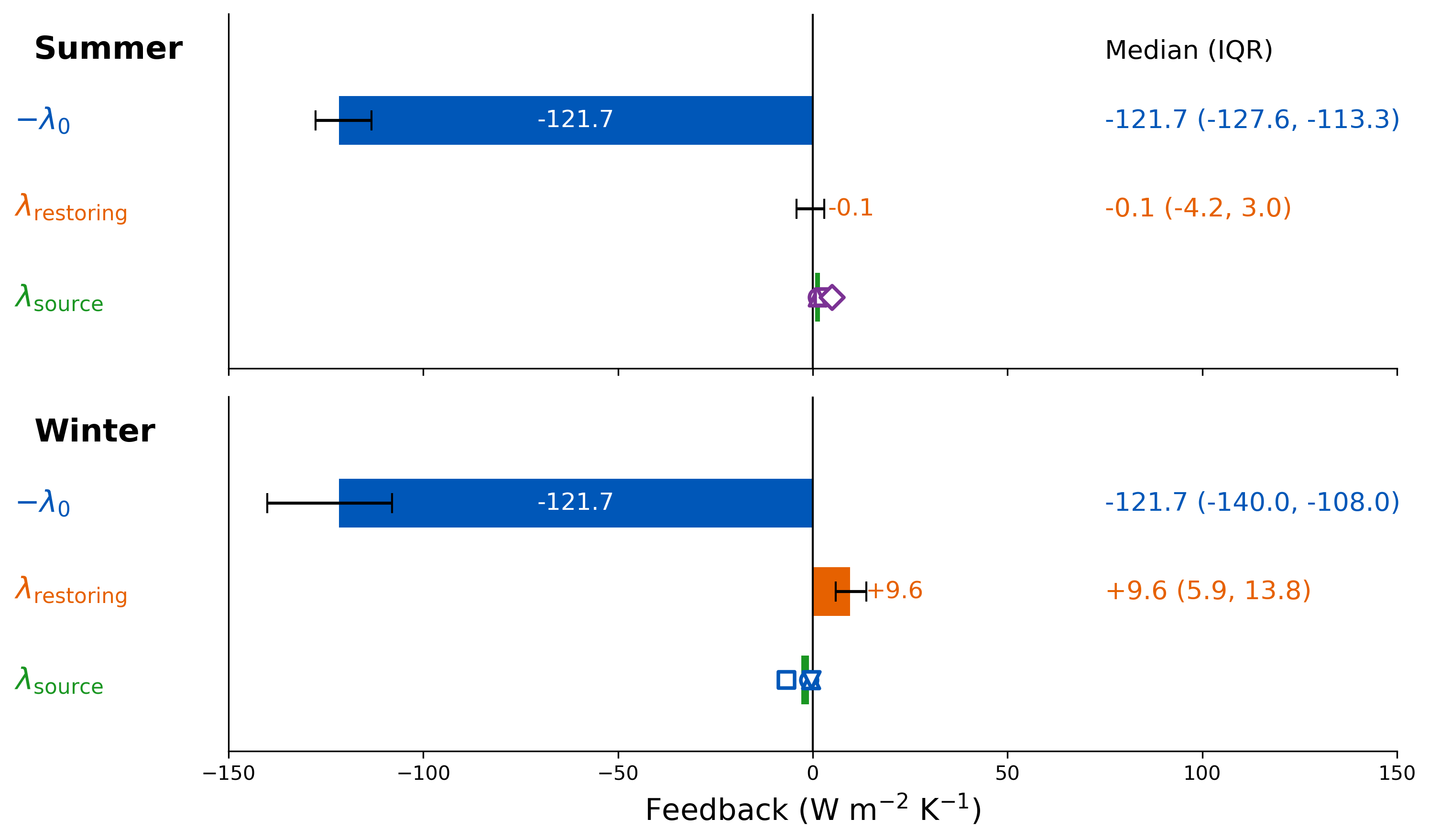
Source feedback
The investigation of source feedback has been enabled primarily by coupling BEMs with urban land surface models, either driven by prescribed atmospheric forcing or coupled with atmospheric models. Examples include Multi-Layer Urban Canopy Model (CM)-BEM (Kikegawa et al. 2003), Building Effect Parameterization (BEP)-BEM (Salamanca et al. 2010), Town Energy Balance (TEB)-BEM (B. Bueno et al. 2012), Urban Tethys & Chloris (UT&C)-BEM (Meili et al. 2025), SLUCM-BEM (Takane et al. 2024), and SLUCM-EnergyPlus (Vahmani et al. 2022). These coupled modeling tools have been widely used to examine interactions among urban microclimate, building energy use, and anthropogenic heat fluxes at city scales (Ohashi et al. 2007; Munck et al. 2013; Salamanca et al. 2014; Takane et al. 2017, 2019, 2022; Xu et al. 2018; Vahmani et al. 2022). More recently, global models have begun to connect climate change, cooling and heating energy demand, and anthropogenic heat emissions in cities (X. C. Li, Zhao, Oleson, et al. 2024; X. C. Li, Zhao, Qin, et al. 2024); parameterizations have been developed to link transportation-related anthropogenic heat fluxes with urban climate (Sun et al. 2026); and attention has expanded to emerging energy-system transitions such as the deployment of air-source heat pumps, the broader electrification of building heating, and heat pump water heaters (Meyer et al. 2024; Takane et al. 2024; Xie et al. 2024; Yamaguchi et al. 2025).
These studies provide the conceptual and modeling basis for treating anthropogenic heat fluxes as temperature dependent and many have expressed this dependence in terms of energy demand amplification or temperature sensitivity of energy demand (Kondo and Kikegawa 2003; Kikegawa et al. 2006; Krpo et al. 2010; Salamanca et al. 2012; Takane et al. 2019, 2024; Nakajima et al. 2022; Takane et al. 2023). Although these studies generally do not characterize source feedback using explicit feedback parameters or gain factors, their reporeted energy demand sensitivities can, in principle, be translated into the source feedback parameter \(\lambda_{\mathrm{source}}\), as shown below, provided the underlying assumptions are carefully considered. Some studies also quantify associated CO\(_2\) emissions (e.g., Yamaguchi et al. 2025), but this pathway is distinct from the source feedback considered here, which describes the local feedback between urban temperature, energy demand, and anthropogenic heat fluxes. By contrast, the pathway through which rising urban temperatures increase CO\(_2\) emissions, which in turn affect the global climate through radiative forcing, operates over much larger spatial and temporal scales and is therefore not considered here.
Ginzburg and Demchenko (2017) was among the first to frame the feedback between urban temperature, energy consumption, and anthropogenic heat flux using the concept of a gain factor (\(g_A\)). In the notation of the present review, this gain factor can be written as \(g_A \equiv \lambda_\text{source} S_0 \equiv \lambda_\text{source}/\lambda_0\). Unlike the framework developed here, which focuses on canopy air temperature, Ginzburg and Demchenko (2017) developed a similar framework for surface temperature by introducing anthropogenic heat flux into the urban surface energy balance equation (Eq. (1)). Although their framework focused on surface temperature and did not explicitly include restoring feedbacks, their estimates of \(\lambda_0\) and \(\lambda_\text{source}\) remain useful for understanding the importance of source feedback.
Neglecting ground heat flux and assuming a very large Bowen ratio so that latent heat flux can also be neglected, Ginzburg and Demchenko (2017) estimated a baseline feedback parameter (\(-\lambda_0\)) of order \(-100\) to \(-10\) W m\(^{-2}\) K\(^{-1}\) under what they called the maximum-advection limit. In this limit, local surface energy perturbations are rapidly removed by radiative and turbulent sensible heat exchange before substantially modifying the overlying atmosphere. In the minimum-advection limit, where the atmosphere is represented as a single equilibrating layer, the baseline feedback parameter (\(-\lambda_0\)) becomes much smaller, approximately \(-1.8\) W m\(^{-2}\) K\(^{-1}\). Demchenko and Ginzburg (2018) later showed that these limiting regimes represent opposite ends of a spectrum controlled by the horizontal length scale of anthropogenic heat forcing relative to the atmospheric thermal adjustment length. The maximum-advection estimate is broadly consistent with the domain-median baseline feedback parameter of approximately \(-120\) W m\(^{-2}\) K\(^{-1}\) obtained by L. Wang et al. (2023), which is notable because the two studies differ substantially, with one focusing on surface temperature in an idealized analytical model and the other on canopy air temperature in an UCM.
Ginzburg and Demchenko (2017) then estimated the source feedback parameter \(\lambda_\text{source}\) from empirical energy demand–temperature relations. For the heating seasons in Moscow, they obtained \(\lambda_\text{source} \approx -0.93\) W m\(^{-2}\) K\(^{-1}\), where the negative sign indicates that warmer conditions reduce heating demand. Following the same approach, \(\lambda_\text{source}\) can be estimated from other published work, for example approximately \(-6.8\) W m\(^{-2}\) K\(^{-1}\) in Toulouse, France (Pigeon et al. 2007) and \(-0.445\) to \(-0.385\) W m\(^{-2}\) K\(^{-1}\) in St. Petersburg, Russia (Ginzburg et al. 2021). Such estimates, however, require caution because the regression slope of an empirical energy demand–temperature relation does not necessarily correspond to the partial derivative defining \(\lambda_\text{source}\). This distinction is discussed further in Section Future outlook.
An alternative approach is to use BEM simulations (e.g., Bruno Bueno et al. 2012; Takane et al. 2019; X. C. Li, Zhao, Qin, et al. 2024) rather than empirical energy demand–temperature relations. In these models, building energy demand and the associated anthropogenic heat fluxes respond to evolving meteorological and climate conditions, allowing the temperature response of \(Q_F\) to be diagnosed directly from simulations. For example, Bruno Bueno et al. (2012) found that residential cooling energy demand increased by approximately 5% per 1 K increase in maximum nighttime UHI intensity. Combined with their simulated \(Q_F\) of approximately 55 W m\(^{-2}\) in residual area, this implies a source feedback parameter of about 2.75 W m\(^{-2}\) K\(^{-1}\), assuming that anthropogenic heat flux scales proportionally with cooling energy demand. Similarly, Takane et al. (2019) and X. C. Li, Zhao, Qin, et al. (2024) conducted simulations under future warming scenarios, although at vastly different spatial scales. For Osaka at 14:00 local time in August, the diagnosed source feedback parameters were 1.27 and 3.32 W m\(^{-2}\) K\(^{-1}\) for office and residential areas, respectively, with the office estimate including only the sensible component (Takane et al. 2019). At the global annual mean scale, the reported source feedback parameters were approximately 0.02–0.05 W m\(^{-2}\) K\(^{-1}\) for cooling and \(-0.4\) to \(-0.3\) W m\(^{-2}\) K\(^{-1}\) for heating, which depend strongly on the assumed Shared Socioeconomic Pathway (X. C. Li, Zhao, Qin, et al. 2024). However, because temperature changes in many such simulations are accompanied by changes in other meteorological variables, the diagnosed source feedback parameters may not correspond to strict partial derivatives that define \(\lambda_{source}\).
As a general rule of thumb, Ginzburg and Demchenko (2017) combined representative temperature sensitivities of energy demand, approximately 5% K\(^{-1}\) for heating and 3% K\(^{-1}\) for cooling, with typical anthropogenic heat fluxes for London (20 W m\(^{-2}\)) and Tokyo (60 W m\(^{-2}\)) (Allen et al. 2011), yielding estimated source feedback parameters of roughly \(\lambda_\text{source} \sim 0.6\)–1.8 W m\(^{-2}\) K\(^{-1}\) during warm seasons and \(\lambda_\text{source} \sim -3\) to \(-1\) W m\(^{-2}\) K\(^{-1}\) during cold seasons (Figure 5). The assumed temperature sensitivities of energy demand are broadly consistent with the literature values as reviewed elsewhere (Santamouris et al. 2015). Combining these source feedback parameters with \(\lambda_0\) shows why source feedback can become important under certain conditions. For example, if \(\lambda_0 \sim 10\) W m\(^{-2}\) K\(^{-1}\) under weak-ventilation conditions, then \(\lambda_\text{source} \sim 1.8\) W m\(^{-2}\) K\(^{-1}\) implies \(g_A=\lambda_\text{source}/\lambda_0 \sim 0.18\), corresponding to an amplification of the reference temperature response by about 20%.
Building on this gain-factor perspective, Kikegawa et al. (2022) were among the first to apply it to analyzing results from coupled UCM-BEM simulations, using Osaka as a case study. They separately estimated \(\lambda_{source}\) and \(\lambda_0\) (or \(S_0\)), the two quantities that determine the gain factor. They used two energy-conserving simulations: a weekdays-run, in which all days were treated as weekdays in urban energy-consumption schedules, and a holidays-run, in which holiday or weekend schedules were imposed. The source feedback parameter \(\lambda_\text{source}\) was estimated from the regression of \(Q_F\) against \(T\) in the weekdays-run, while \(S_0\) was estimated from the regression of \(\Delta T\) against \(\Delta Q_F\), where \(\Delta\) was taken as the difference between the weekdays-run and the holidays-run. Again, the extent to which these regression-based diagnostics correspond to the formal feedback parameters is discussed further in Section Future outlook.
Kikegawa et al. (2022) illustrated the estimates for three Osaka districts in their Figure 15. The commercial district had a much larger source feedback parameter, with \(\lambda_\text{source}=6.137\) W m\(^{-2}\) K\(^{-1}\), but also a larger \(\lambda_0=62.5\) W m\(^{-2}\) K\(^{-1}\). By contrast, the residential examples had smaller \(\lambda_\text{source}\) and \(\lambda_0\), especially the R7 district, where \(\lambda_\text{source}=0.787\) W m\(^{-2}\) K\(^{-1}\) and \(\lambda_0=2.71\) W m\(^{-2}\) K\(^{-1}\). When averaged over the daytime period and across urban grids, Kikegawa et al. (2022) reported \(\lambda_\text{source}\) of 4.87 W m\(^{-2}\) K\(^{-1}\) for commercial areas and 1.15–1.42 W m\(^{-2}\) K\(^{-1}\) for residential areas. The corresponding \(\lambda_0\) were approximately 50 W m\(^{-2}\) K\(^{-1}\) for commercial grids and 6.25–7.14 W m\(^{-2}\) K\(^{-1}\) for residential grids. These two quantities imply gain factors of about 10% in commercial areas and 20% in residential areas.
Summary
Taken together, these pioneering studies suggest an emerging picture of anthropogenic heat feedback. The available estimates indicate that both source and restoring feedback parameters are generally of order 10 W m\(^{-2}\) K\(^{-1}\) or smaller, while estimates of the baseline feedback parameter span a much wider range across the available studies. In the long-term climatological estimates of L. Wang et al. (2023), the baseline feedback parameter is of order 100 W m\(^{-2}\) K\(^{-1}\), comparable to the upper end of the maximum-advection range estimated by Ginzburg and Demchenko (2017). Substantially smaller baseline feedback parameters have also been reported, for example, by Kikegawa et al. (2022) for a residential district at 16:00 local time in summer, suggesting that the diagnosed baseline feedback parameter depends strongly on the temporal and spatial scales considered.
These findings should, however, be regarded as preliminary, given the small number of studies and their differences in models, assumptions, diagnostic methods, and, importantly, the temporal and spatial scales over which the feedback parameters are diagnosed. Establishing whether these patterns generalize across cities, climates, and modeling systems requires more systematic investigations.
Future outlook
The literature synthesized in this review reveals a clear imbalance: substantial progress has been made in quantifying the forcing and documenting its effects in applied contexts, but less generalizable understanding has emerged regarding the urban temperature response to that forcing and the feedbacks that amplify or damp the response. This imbalance is reflected in the textbook by Oke et al. (2017), which devotes substantial attention to the magnitude, sources, and estimation of anthropogenic heat flux, but only a brief discussion of its climatic significance. This disparity does not necessarily imply that the climatic effects of anthropogenic heat flux have received little attention; rather, it suggests that the large body of observational and modeling work has primarily addressed specific cities, applications, and modeling systems, making it difficult to extract broader physical understanding.
Interestingly, however, a sensitivity concept was hinted at in the discussion of Oke et al. (2017), who noted that “the atmospheric thermal response (increase in air temperature per unit energy flux density) depends on the whole surface energy balance … and the mixing efficiency of the air in the roughness sublayer.” In retrospect, this statement foreshadowed both the sensitivity concept and the role of \(C_{ha}\) and \(C_{hs}\) in controlling the sensitivity. The framework developed in this review formalizes this insight and brings reference sensitivity, restoring feedback, and source feedback, which have been treated separately and implicitly in some previous work, under a unified framework. The framework also clearly distinguishes forcing-based sensitivity from effective sensitivity.
Looking ahead, the field should advance across all three components of the framework. Better estimates and representations of anthropogenic heat forcing remain essential, but equally important are more rigorous characterization of sensitivity and more systematic diagnosis of feedbacks. The following subsections discuss future priorities for advancing each of these three components.
Quantifying and representing anthropogenic heat forcing
For anthropogenic heat forcing, the next challenge is not simply to produce more \(Q_F\) estimates, but to make them standardized, accompanied by quantified uncertainties, and physically usable in numerical models. This requires two complementary efforts: standardizing and benchmarking \(Q_F\) datasets, and representing \(Q_F\) as a physically structured forcing.
Standardization, benchmarking, and scenario-based future \(Q_F\) datasets
Current global and regional \(Q_F\) datasets differ in units, spatiotemporal resolution, sectoral decomposition, and reporting conventions. In addition, deterministic estimations of \(Q_F\) should provide adequate uncertainty quantification. Establishing community standards for data formats, metadata, sector definitions, reporting conventions, and uncertainty quantification would therefore facilitate localized evaluations in data-scarce regions, comparison among datasets, and streamlined applications in weather, climate, and earth system models. Similar to the role played by the Emissions Database for Global Atmospheric Research (EDGAR) (Crippa et al. 2018) for atmospheric emissions, an operational and regularly updated global anthropogenic heat forcing database would provide a common resource for numerical modeling.
Future research should also place greater emphasis on intercomparison among independent estimation methods. Comparisons among inventories, residual surface energy balance approaches, building energy models, remote sensing products, and eddy covariance observations in well-observed cities provide opportunities to quantify uncertainties in \(Q_F\) and identify method-specific biases. The study by Chow et al. (2014) illustrates the value of such benchmark studies, showing that multiple independent approaches can converge to consistent estimates while also identifying their respective strengths and weaknesses. Expanding similar benchmarking efforts across diverse climates, urban forms, and socioeconomic settings would provide a stronger foundation for evaluating anthropogenic heat flux data products.
Sailor (2011)’s vision of community-scale anthropogenic heat forcing datasets for atmospheric modeling has largely been realized for historical and present-day conditions, although these products still require further standardization, comprehensive benchmarking, and systematic uncertainty quantification. The next challenge is to move toward scenario-based future \(Q_F\) datasets (Varquez et al. 2021) that describe how anthropogenic heat flux may evolve under continued urbanization, socioeconomic development, technological change, and climate-driven energy demand. Many sectoral components of \(Q_F\), including industrial emissions, transportation, and metabolic heat release, have yet to be distinctly provided for future projection purposes. Developing, maintaining, and properly documenting such datasets would allow anthropogenic heat flux estimates to be more consistent with changes in climate, urbanization, and energy systems; and always up-to-date with advancing computational approaches.
Source and release pathway representation
Recent advances have enabled explicit representation of building, transportation, industrial, and metabolic heat sources, as well as dynamic coupling between BEMs, traffic modules, and urban land surface models. Future developments should continue this transition from prescribing total anthropogenic heat fluxes toward physically based representations of individual source sectors.
Of equal importance is the pathway through which anthropogenic heat enters the urban climate system, which may be related to, but is not necessarily identical to, the source sector. Heat released at street level by vehicles, rejected above roofs by HVAC systems, emitted from industrial stacks, or discharged from underground infrastructure can produce different climate responses even with the same total \(Q_F\) (Kikegawa et al. 2003; D. Li et al. 2024; Zhang et al. 2024). This issue was already recognized by Oke (1974) and Sailor (2011), yet comparatively little progress has been made in representing these release pathways explicitly. Developing data and parameterizations for these release pathways, including their vertical distribution and physical characteristics, should therefore become a priority for next-generation \(Q_F\) datasets and urban climate models.
Defining and characterizing anthropogenic heat sensitivity
Compared with anthropogenic heat forcing, anthropogenic heat sensitivity remains less well constrained. Observational estimates are still very limited, while existing model estimates are affected by inconsistent definitions and methodological differences across studies. Although pioneering studies have begun to clarify the typical magnitude, variability, and uncertainty of anthropogenic heat sensitivity, major gaps remain in how sensitivity is defined, computed, and interpreted, and in whether estimates obtained for one model, location, or spatial and temporal scale are applicable to others. Future progress therefore requires stronger observational constraints, greater consistency in how anthropogenic heat sensitivity is defined and reported, and a more systematic understanding of its variability and uncertainty.
In this review, anthropogenic heat sensitivity is interpreted as a scalar relationship between anthropogenic heat flux and an equilibrium temperature response. In reality, however, both \(\Delta Q_F\) and \(\Delta T\) vary spatially and temporally, and a temperature change at a given location and time is not necessarily driven solely by the anthropogenic heat flux change at that same location and time. Diagnosing a scalar anthropogenic heat sensitivity therefore depends critically on how the anthropogenic heat flux and response are averaged over specified spatial domains and temporal windows. This raises two important questions. First, how does the diagnosed sensitivity depend on the spatial and temporal scales over which the forcing and response are averaged? Second, does the diagnosed sensitivity depend on the spatial and temporal pattern of anthropogenic heat forcing within the averaging domain and window? These questions are discussed below.
Characterizing scale dependence
Scale dependence first arises from the temporal averaging window, as different components of the urban climate system adjust to anthropogenic heat flux perturbation over different timescales. Canopy air temperature may adjust rapidly toward a quasi-equilibrium state, but other processes that influence anthropogenic heat sensitivity may operate on longer timescales. Turbulent exchange between the canopy layer and the overlying atmosphere may act over seconds to minutes, whereas surface temperature and boundary-layer temperature adjustments, and source feedbacks involving building energy use can evolve over much longer periods.
A quasi-equilibrium sensitivity can therefore be meaningful for canopy air temperature when the averaging timescale is long compared with the adjustment timescale of the canopy air subsystem, a condition that is often attainable. However, it should not automatically be interpreted as the equilibrium response of the entire urban surface or atmosphere, which generally requires longer timescales. This distinction is especially important for simulations lasting only several hours or a single day, in which canopy air temperature may approach quasi-equilibrium while slower surface, boundary-layer, and mesoscale adjustments remain incomplete. When the averaging timescale is longer than the canopy-air adjustment timescale but shorter than the adjustment timescales of these slower processes, the diagnosed sensitivity may continue to evolve as those processes respond, manifested as transient or only partially realized feedbacks.
The spatial averaging domain is equally important because anthropogenic heat forcing and temperature response are generally not co-located. Horizontal advection, turbulent transport, and mesoscale circulations allow anthropogenic heat emissions released in one location to influence temperatures elsewhere. Ideally, the averaging domain should encompass the spatial footprint of the temperature response induced by the anthropogenic heat perturbation. In practice, however, this response footprint is rarely quantified and likely depends on factors such as atmospheric stability, wind, boundary-layer depth, urban morphology, and the spatial distribution of anthropogenic heat emissions. Different averaging domains may therefore capture different fractions of the total temperature response, making sensitivities diagnosed at different spatial scales not directly comparable.
Future studies should therefore systematically quantify how diagnosed sensitivities vary with the temporal averaging window and spatial averaging domain, and determine whether they converge beyond characteristic temporal or spatial scales. Such analyses would help establish the relationships among instantaneous, hourly, daily, seasonal, and longer-term sensitivities, as well as among canopy-, neighborhood-, city-, and regional-scale sensitivities. Future studies should also extend the forcing–response–feedback framework to other control volumes and state variables (e.g., the surface–canopy–boundary-layer continuum), with explicit consideration of the spatial scale of the forcing perturbation and the adjustment time scale of the system (Yang et al. 2016; Demchenko and Ginzburg 2018; Xue et al. 2020; Khanh et al. 2025).
Characterizing pattern dependence
Anthropogenic heat sensitivity may depend not only on the mean anthropogenic heat forcing averaged over the selected temporal window and spatial domain, but also on how that forcing is distributed in time and space. Temporally, the same mean anthropogenic heat release may occur as a nearly constant background forcing, exhibit strong diurnal variations, or be concentrated during short episodes associated with traffic, building cooling demand, or industrial activity. Spatially, the same domain-mean anthropogenic heat flux may be concentrated within dense urban cores, distributed across residential neighborhoods, or aligned along transportation corridors.
Future studies should determine whether, and under what conditions, temporal and spatial forcing patterns affect anthropogenic heat sensitivity. Rather than relying only on observed patterns of anthropogenic heat flux, idealized experiments could systematically vary the structure of the forcing while holding the total heat input fixed. This would help characterize the response function of the urban climate system and test whether centralized, distributed, corridor-like, constant, diurnally varying, or episodic forcing produces meaningfully different sensitivities. Characterizing the role of forcing pattern would help determine when the mean forcing is sufficient for defining anthropogenic heat sensitivity and when more temporally or spatially resolved descriptions are needed.
If anthropogenic heat sensitivity depends strongly on the spatial or temporal pattern of the forcing, a single scalar sensitivity based on mean \(\Delta Q_F\) may be insufficient to characterize the response. More general formulations could instead adopt a source–receptor perspective, representing the temperature response at a given location and time as a function of anthropogenic heat flux across different locations and times. This would allow \(\Delta Q_F\) and \(\Delta T\) to be evaluated over different spatial domains and temporal windows and could better capture transport, storage, and delayed adjustment. Developing and testing such formulations will require substantial future work, but they may ultimately provide a more general framework for characterizing anthropogenic heat sensitivity across scales.
Diagnosing and understanding anthropogenic heat feedbacks
Despite increasing recognition of the importance of anthropogenic heat feedbacks, their quantitative understanding remains at a much earlier stage than that of anthropogenic heat forcing and sensitivity. Many studies have examined the effects of feedbacks through coupled simulations, often by comparing temperature responses with and without particular feedback pathways, yet relatively few have attempted to quantify the role of these feedbacks using explicit feedback parameters (or equivalent gain factors). Future progress therefore requires moving beyond documenting the temperature and other effects of feedbacks toward diagnosing, isolating, and comparing feedback parameters across different models, cities, climates, and temporal/spatial scales.
Diagnosing feedback parameters
A first priority is to define feedback parameters in ways that can be diagnosed consistently from model outputs. Studies such as Kikegawa et al. (2022) and L. Wang et al. (2023) represent important steps in this direction because they estimate feedback parameters directly rather than only reporting the temperature effects associated with particular feedback pathways. Nevertheless, diagnosing feedback parameters is not always straightforward. For example, Kikegawa et al. (2022) estimated \(\lambda_{\rm source}\) from the regression of \(Q_F\) against \(T\) within their weekdays-run. However, because temperature covaries with other meteorological controls on building energy demand and thus \(Q_F\), this regression should be interpreted as an operational diagnostic rather than a strict estimate of the partial derivative defined in the present framework. Likewise, regression-based estimates from empirical energy demand-temperature relations (e.g., Pigeon et al. 2007; Ginzburg et al. 2021) and other building energy simulations (e.g., Takane et al. 2019; X. C. Li, Zhao, Qin, et al. 2024) generally do not isolate temperature effects with all other factors held fixed. Similarly, \(S_0\) is formally defined as the reference sensitivity in the absence of source and restoring feedbacks, whereas many estimates, including that of Kikegawa et al. (2022), are derived from simulations that retain both feedbacks. Overall, such estimates should be interpreted as operational diagnostics rather than strict representations of the formal quantities defined in the present framework.
A related challenge concerns the definition of forcing-based sensitivity in studies that include source feedback. As emphasized in Sections Sensitivity and Feedback, once anthropogenic heat flux is allowed to respond to temperature, separating the anthropogenic heat forcing from the temperature-dependent source-feedback contribution is not always straightforward. For example, the total anthropogenic heat flux predicted by a BEM generally contains both a reference heat release that acts as the forcing and an additional temperature-dependent contribution arising from source feedback. One conceptually straightforward way to isolate the source-feedback contribution would be to compare a fully coupled simulation with a counterfactual simulation in which the release of anthropogenic heat into the atmosphere is suppressed. However, suppressing anthropogenic heat release while continuing to simulate building energy consumption effectively introduces an energy sink, rendering the coupled building–atmosphere energy budget physically inconsistent (Kikegawa et al. 2022).
This methodological tension reflects different objectives in urban climate modeling and climate feedback analysis, but it also points to a broader opportunity for future research. Methodologies developed in climate science for diagnosing forcing, sensitivity, and feedback provide a valuable conceptual framework for interpreting coupled urban-energy simulations, but they must be adapted to account for the physical constraints of these models. Future work should therefore develop diagnostics and experimental designs that isolate feedback parameters without sacrificing the physical consistency of coupled building–atmosphere interactions.
Understanding feedback parameters
Substantially more work is needed to understand how feedback parameters vary across space, time, urban form, and background meteorological conditions. Current knowledge remains limited because only a small number of studies have quantified these parameters explicitly, and some feedbacks have not yet been quantified at all.
A central priority is to quantify the variability of the baseline feedback parameter because it sets the reference against which source and restoring feedbacks are evaluated: the same feedback parameter can imply very different gain factors depending on the magnitude of \(\lambda_0\). Future work should systematically characterize the variability of \(\lambda_0\) and identify the physical processes that control it.
Existing studies of restoring feedback have focused primarily on processes within the urban canopy (L. Wang et al. 2023), although D. Li et al. (2024) extended the analysis to include atmospheric temperature adjustments in land–atmosphere coupled simulations. Restoring feedbacks associated with broader boundary-layer adjustment, horizontal advection, and mesoscale circulations, however, remain largely unquantified, as do the characteristic timescales over which these feedbacks develop and become fully realized. Extending the framework across the entire urban boundary layer and to larger spatial and temporal scales therefore remains an important next step.
Although the sign of source feedback appears to be relatively well established in many conventional heating and cooling systems, quantitative estimates remain limited, leaving its dependence on climate, building characteristics, energy systems, technology, and human behavior largely unknown. Emerging technologies may also introduce feedback pathways beyond those captured by the conventional definition of anthropogenic heat flux. For example, air-source heat pumps are expected to reduce wintertime \(Q_F\) in the traditional sense. However, colder conditions can increase heating demand and associated heat extraction from the outdoor air, thereby forming an amplifying local winter-cooling pathway in building–atmosphere heat exchange (Meyer et al. 2024; Takane et al. 2024; Xie et al. 2024). This pathway is conceptually similar to a positive source feedback, although it has not generally been quantified explicitly using a feedback parameter. Quantifying both conventional source feedbacks and these new feedback pathways will be essential for projecting future urban climate responses as cities electrify, building technologies improve, cooling demand increases, and patterns of energy consumption change.
Beyond linear feedback theory
Finally, the forcing–response–feedback framework developed in this review is based on a local linearization of the urban climate system, whose range of validity requires much more systematic investigation. Existing studies provide mixed evidence. Offline land-model simulations have reported declining sensitivities under large anthropogenic heat flux perturbations (L. Wang et al. 2023), whereas regional climate simulations have found similar sensitivities over a range of \(Q_F\) values, implying approximately linear temperature responses (D. Li et al. 2024). More recently, idealized large-eddy simulations under calm conditions demonstrated power-law rather than linear scaling between urban temperature and surface heat flux, indicating nonlinearities arising from the atmospheric response (O’Brien et al. 2026). Similarly, global modeling studies have suggested that the strength of source feedback may itself change under a warming climate (X. C. Li, Zhao, Qin, et al. 2024). Together, these results suggest that the validity of local linearization depends on both the magnitude of the forcing and the state of the urban climate system, and may also depend on the spatial and temporal scales over which the response is considered. Future work should identify the conditions under which linear theory remains applicable, determine when nonlinear behavior becomes important, and develop generalized forcing–response frameworks capable of describing both linear and nonlinear regimes.
Final Remarks
Anthropogenic heat flux (\(Q_F\)) has long been recognized by the urban climate community as an important component of the urban surface energy balance, with potential relevance to the broader climate science community. However, relatively little work has sought to interpret the role of anthropogenic heat flux using the conceptual language of forcing, sensitivity, and feedback that underpins much of modern climate science, as the urban climate community has largely approached anthropogenic heat flux from an applied perspective. This review represents a step toward bridging the gap between applied urban meteorology and climate science by introducing a forcing–response–feedback framework for understanding the temperature effects of anthropogenic heat flux.
A central message of this review is that the climatic significance of anthropogenic heat flux depends not only on the forcing itself, but also on the response of urban temperatures to that forcing and on the feedbacks that amplify or damp the response. Reinterpreting the existing literature through this framework reveals that many seemingly disparate studies share common physical interpretations, while also highlighting ambiguities in the definition and diagnosis of anthropogenic heat sensitivity and feedback parameters that complicate comparisons across studies.
This review synthesizes selected studies that quantify anthropogenic heat sensitivities and feedback parameters, and uses them to distinguish forcing-based sensitivity, effective sensitivity, and reference sensitivity. It also clarifies the differences among baseline, restoring, and source feedbacks. More broadly, it demonstrates how methodologies developed in climate science can provide valuable guidance for interpreting urban climate studies, while also emphasizing the need to adapt these methodologies to accommodate the physical constraints of urban climate models.
Finally, this review suggests that future progress depends not only on improving estimates of anthropogenic heat forcing, but also on systematically quantifying sensitivities and feedbacks across different cities, climates, and modeling frameworks. Developing transferable physical understanding requires giving as much attention to the forcing–response relationship as to the forcing itself. We hope this review demonstrates the value of bringing together concepts from climate feedback theory with urban observations and simulations, and motivates similar efforts in other domains, including urban climate adaptation, where the effects of interventions such as reflective roofs may likewise be interpreted through the lens of forcing, sensitivity, and feedback (Li 2025).
Open Research Section
The materials needed to reproduce the corpus assembly and structured extraction are available in Li et al. (2026) and explained in the supporting information. The corpus and its structured extraction can also be browsed through a companion website (https://ah.urbanclimaterisk.group), which supplements the archived materials in Li et al. (2026) but does not replace them as the citable record of the data supporting this review. Data and scripts for reproducing the figures are also available in Li et al. (2026). The global datasets of \(Q_{F}\) presented in Figure 2 are accessible via publicly-available repositories and archives. Specifically, AH4GUC (Varquez et al. 2021), AH-DMSP (Yang et al. 2017), PF-AHF (Jin et al. 2019), and Dong (Dong et al. 2017) are available at https://doi.org/10.6084/m9.figshare.12612458, https://doi.org/10.6084/m9.figshare.c.3647903, https://doi.org/10.6084/m9.figshare.c.4182824, and https://doi.org/10.5281/zenodo.21767353, respectively. Figure 2 uses the 2013 field of the \(0.5^{\circ}\) dataset of Flanner (2009) (AHF_2005-2040_0.5x0.5.nc). That dataset is no longer distributed by its original host, http://www.cgd.ucar.edu/tss/ahf/data/, which went offline in 2024, and it has no persistent identifier of its own; the copy used here was retrieved on 7 August 2026 from the Internet Archive’s capture of 13 April 2012, verified against the checksum that the archive records for that capture, and is redistributed together with its provenance record in Li et al. (2026).
Acknowledgments
We thank Dr. Yukihiro Kikegawa and Dr. Do Ngoc Khanh for their insightful discussions and valuable perspectives. We also thank Xuanzong Zhang for preparing the theory figure and Dr. Linying Wang for generously providing the data used in the feedback synthesis figure. This review was conceived and largely written during DL’s visit to the Institute of Science Tokyo, which was supported by Boston University and the World Research Hub Program of the Institute of Science Tokyo, and benefited greatly from the stimulating discussions and collaborative environment there. DL also acknowledges partial support from the U.S. Department of Energy, Office of Science, as part of research in MultiSector Dynamics, Earth and Environmental System Modeling Program. ACGV acknowledges the support of JSPS Kakenhi grant JP25K00040. TS acknowledges support from the Royal Society–NSFC International Exchanges scheme (Grant No. IEC\NSFC\242040). YT acknowledges support from the Japan Science and Technology Agency (JST) FOREST Program (Grant Number JPMJFR241G, Japan) and the Environment Research and Technology Development Fund (JPMEERF25S12433) of the Environmental Restoration and Conservation Agency provided by the Ministry of the Environment of Japan. JY acknowledges support from the National Natural Science Foundation of China (Excellent Young Scientists Fund, Grant No. 42322903). DJS acknowledges partial support from the U.S. Department of Energy, Office of Science, Office of Biological and Environmental Research’s Urban Integrated Field Laboratories research activity, under Award Number DE-SC0023520.